How to create a choropleth map
A choropleth map is a map in which regions (like states or countries) are filled with colors according to your data. Often, these colors show one number per region – and the darker the color (on a bright background), the higher the number.
This article explains how to build a choropleth map. We'll use the following map of the age structure in Australia as an example. The darker the color, the higher the share of people who are 75 years old or older:

Choosing a map
To create a new choropleth map, click on Create new ❶ > Map ❷ at the top of the Datawrapper app, or go directly here: app.datawrapper.de/create/map and click on Choropleth map ❸.
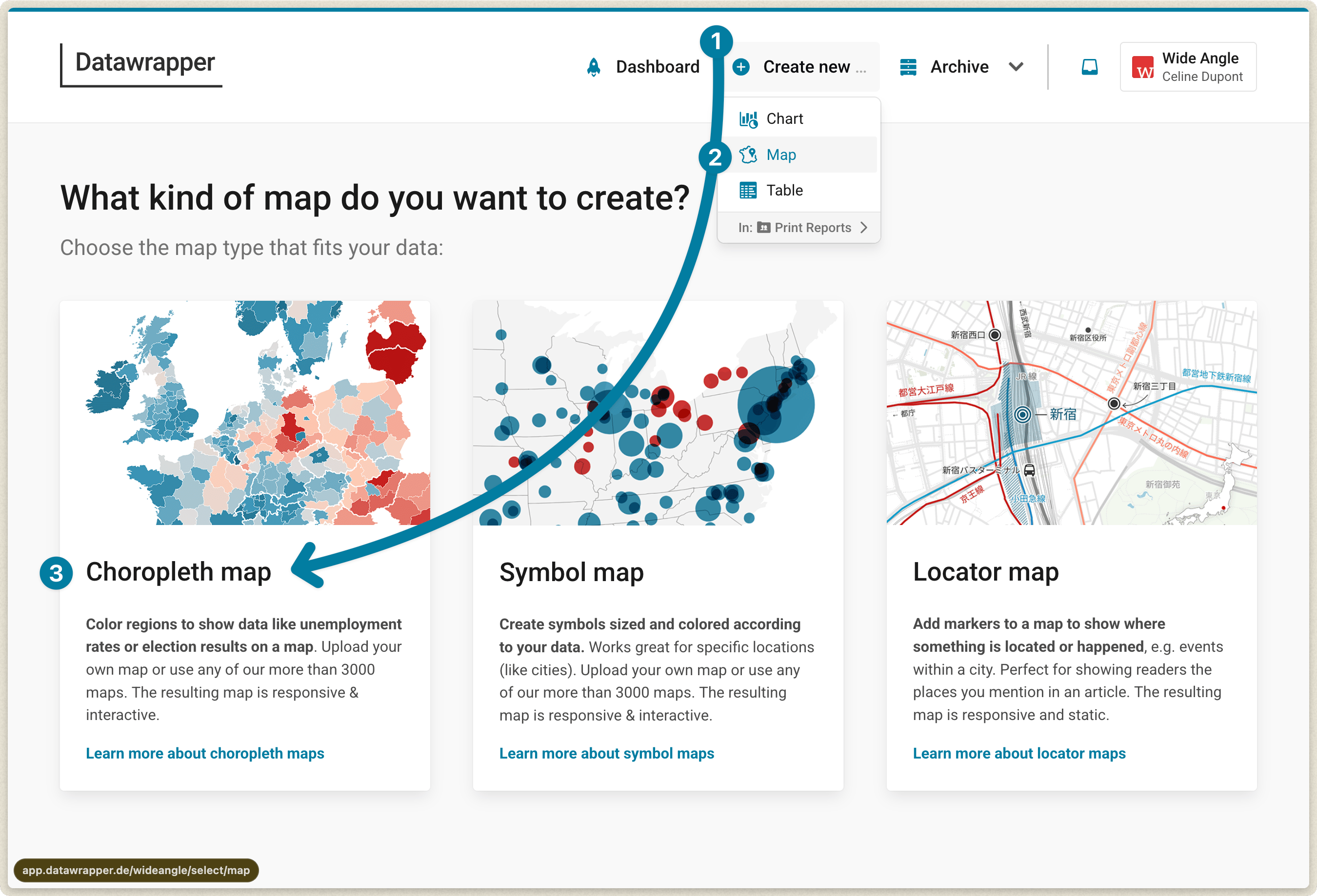
The first thing your choropleth map needs is a basemap.
Even if you know that you want a map of Australia, you can still decide between different levels, e.g. postal areas, suburbs, and electoral districts – and sometimes even different years.
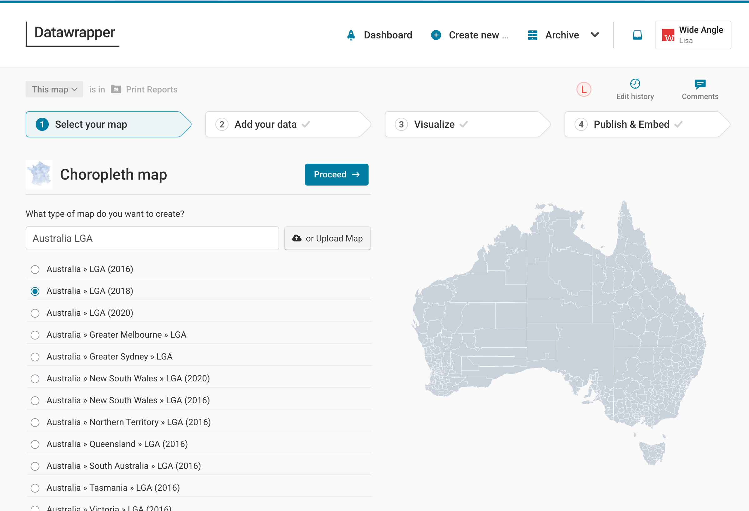
We want a map of Australia's Local Government Areas (LGA), so we'll search for "Australia LGA", click on Australia » LGA and then click Proceed. Learn here how to upload your own map.
Preparing your data
Before we can visualize our age data, we need to bring it into the right format. Datawrapper needs a table with at least two columns:
- The key of each region you want to fill with a color. Most often, that's the name, like county names. But some regions have specific IDs, e.g. the FIPS-Code for counties in the US, or the LGA Code (which we'll use for our map).
- The value for each region. The values can be percentages (43.4%), full numbers (38430), or categories (yes/no/maybe). Our table will have the column called "75 or older" with numerical values: the share of people who are 75 years old or older.
Here is our table. As you can see, we have two more columns, "States" and "LGA name". You can upload as many columns as you like, as long as one of them has a map key and one of them has some kind of value. Extra information like the state can be useful for tooltips, so we want to keep them in our table.
| LGA Code | LGA Name | 75 or older | States |
| 10050 | Albury | 8.12 | New South Wales |
| 10130 | Armidale Regional | 7.94 | New South Wales |
| 10250 | Ballina | 11.84 | New South Wales |
| 10300 | Balranald | 7.78 | New South Wales |
| ... | ... | ... | ... |
Adding your data
Uploading your data
Once you've prepared the data, let's add it to your map! You'll find all the options to do so in the Upload tab in step 2: Add your data:
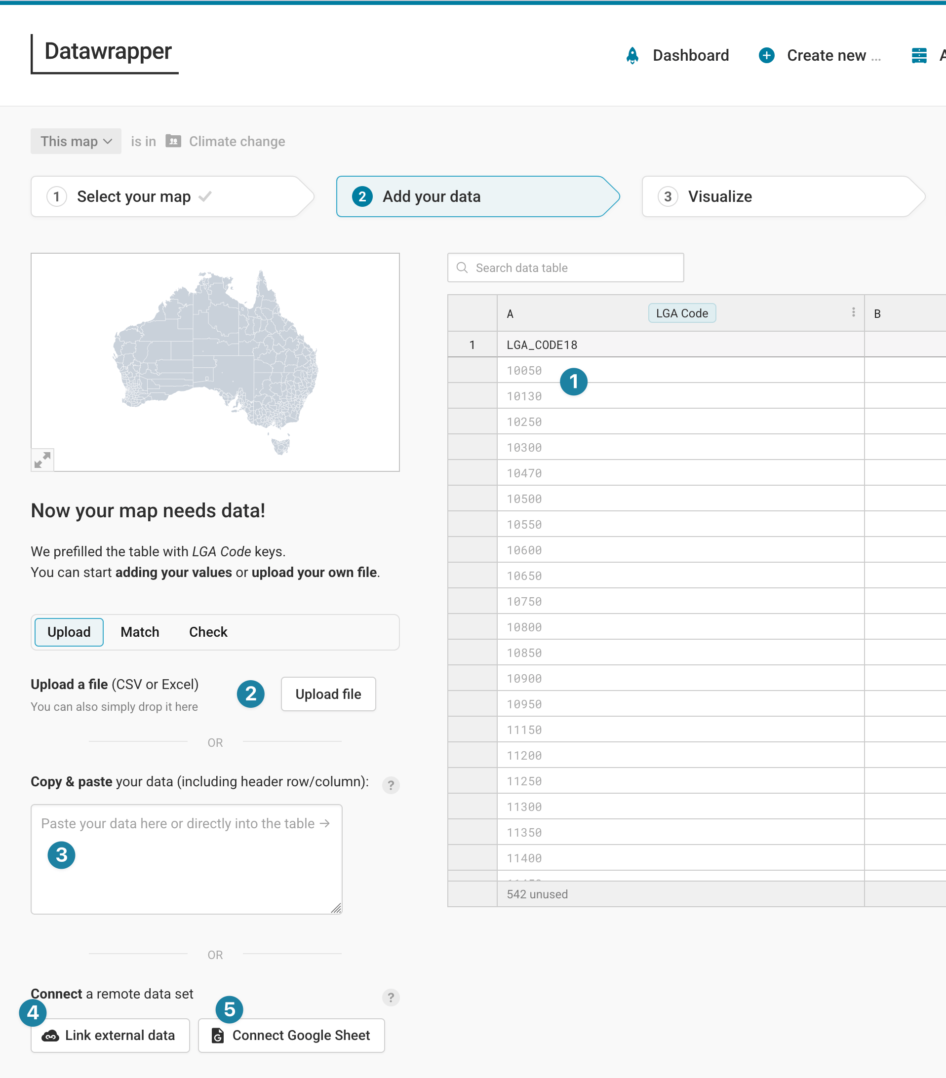
Here are all the ways to import your table:
- Write your values directly into the Datawrapper table. This takes a long time, so this works best for maps with only a few regions.
- Upload a CSV or Excel file. To do so, click on Upload file.
- Copy & paste your data into the text field in the Upload tab, for example, from Excel or Google Sheets. This is the most convenient option for lots of our users.
- Link an external dataset. That's the best option if your data keeps updating (e.g. election results during election night), and you want your embedded map to always show the latest numbers. Learn more about creating live-updating choropleth maps.
- Import a Google Spreadsheet. That's a good option if you or a coworker is changing the data by hand a lot and you want to make sure that your map shows the latest numbers when visualizing it. Learn more about connecting your choropleth map to Google Sheets.
Below all that, you'll find the option to fill the table with random data (if you just want to try out our tool).
Matching your data
Once you upload your data, Datawrapper automatically tries to match your columns with the matching keys it has stored for each map. In the case of the Australia map, Datawrapper accepts the LGA code or the LGA name. We uploaded both, and you can choose either in Match > Matching key.
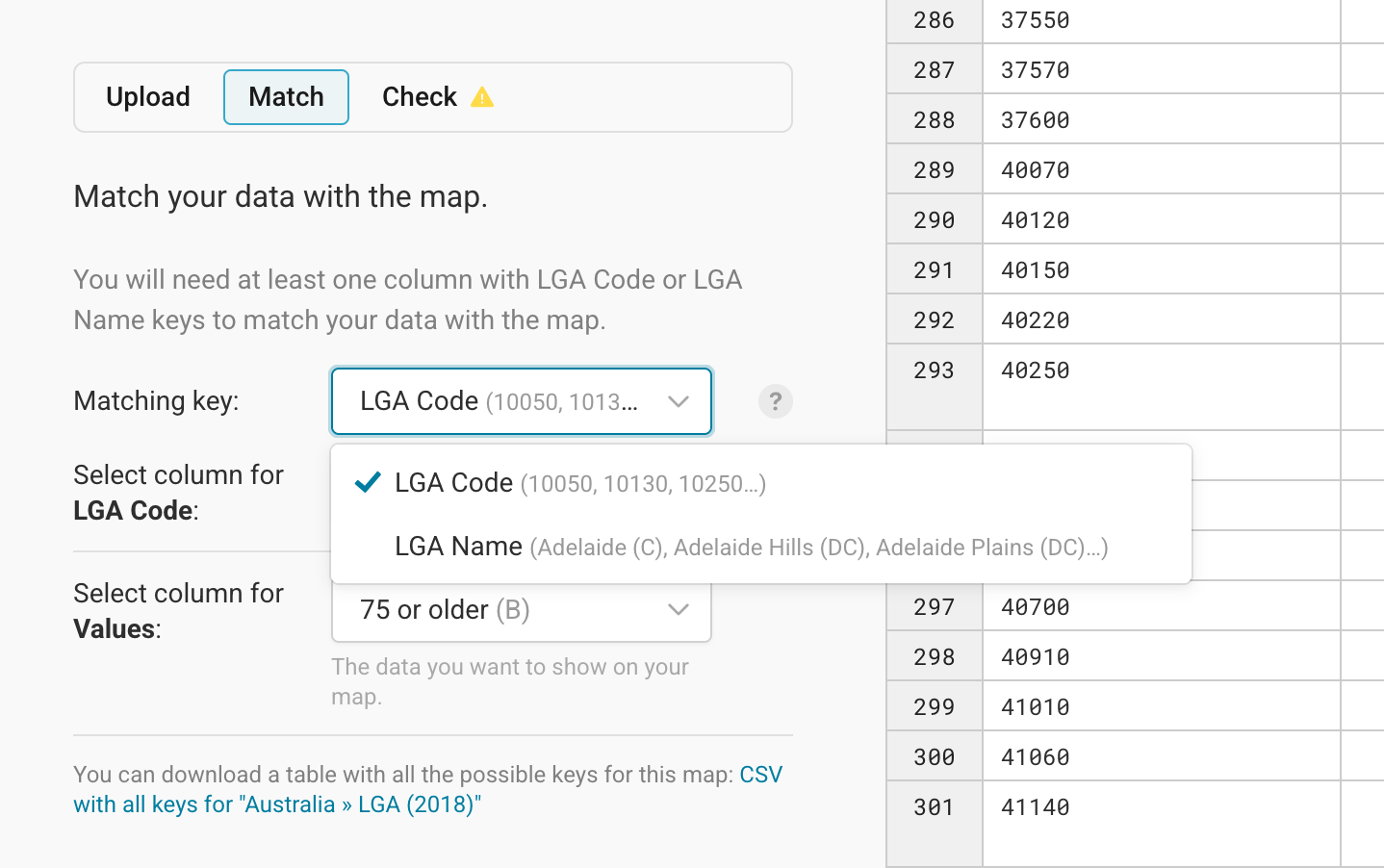
We recommend checking which matching keys are accepted at the beginning of your data preparation process. You can download a CSV with all possible keys for the map directly from the Match tab (see the bottom of the screenshot above).
Names can be fuzzy because they might have abbreviations, extra spaces, more details, etc. So an ID is often the safer bet to make sure that as many areas as possible get matched correctly.
If Datawrapper didn't match your columns correctly, you can select the column that has the matching key (LGA code, in our case) and the columns for values (you can still change this later) yourself in the Match tab.
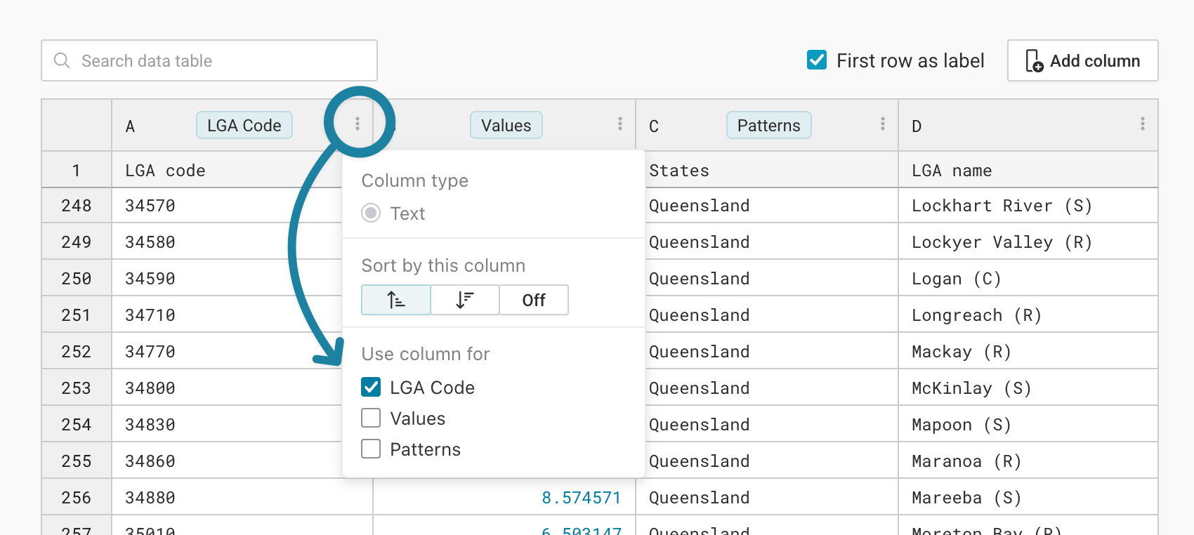
You can also define what your columns should be used for directly in the table. To do so, click on the three dots next to the column ID ("A", "B", etc.), then check any of the check boxes below Use column for:
Checking your data
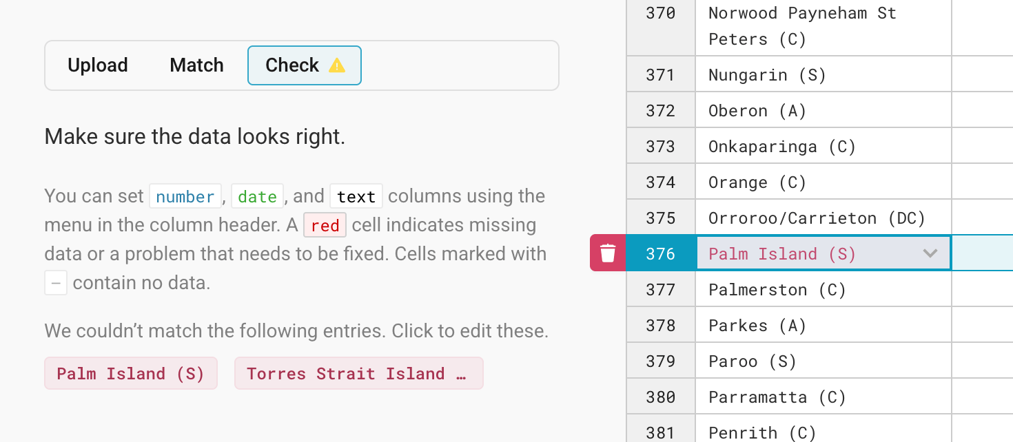
Some of your regions might have a different key in your data than in our map – e.g. "Czechia" instead of "Czech Republic" in a map about Europe. Datawrapper will highlight the regions it couldn't match in your dataset in the Check tab, and lets you correct them.
Click on one of the highlighted entries in the Check tab, and you'll see the corresponding row in the table with all yet-unmatched regions. Here's what that looks like if we choose the LGA names as our matching keys:
If Datawrapper (and you) can't find the correct matching key for a region, it will be ignored in the final map. To delete a row, click on the row number and the little trash icon that appears next to it:
If you successfully imported and matched the data, click on Proceed to go to step 3: Visualize. Here, you'll notice three tabs: Refine, Annotate, and Layout.
Resizing
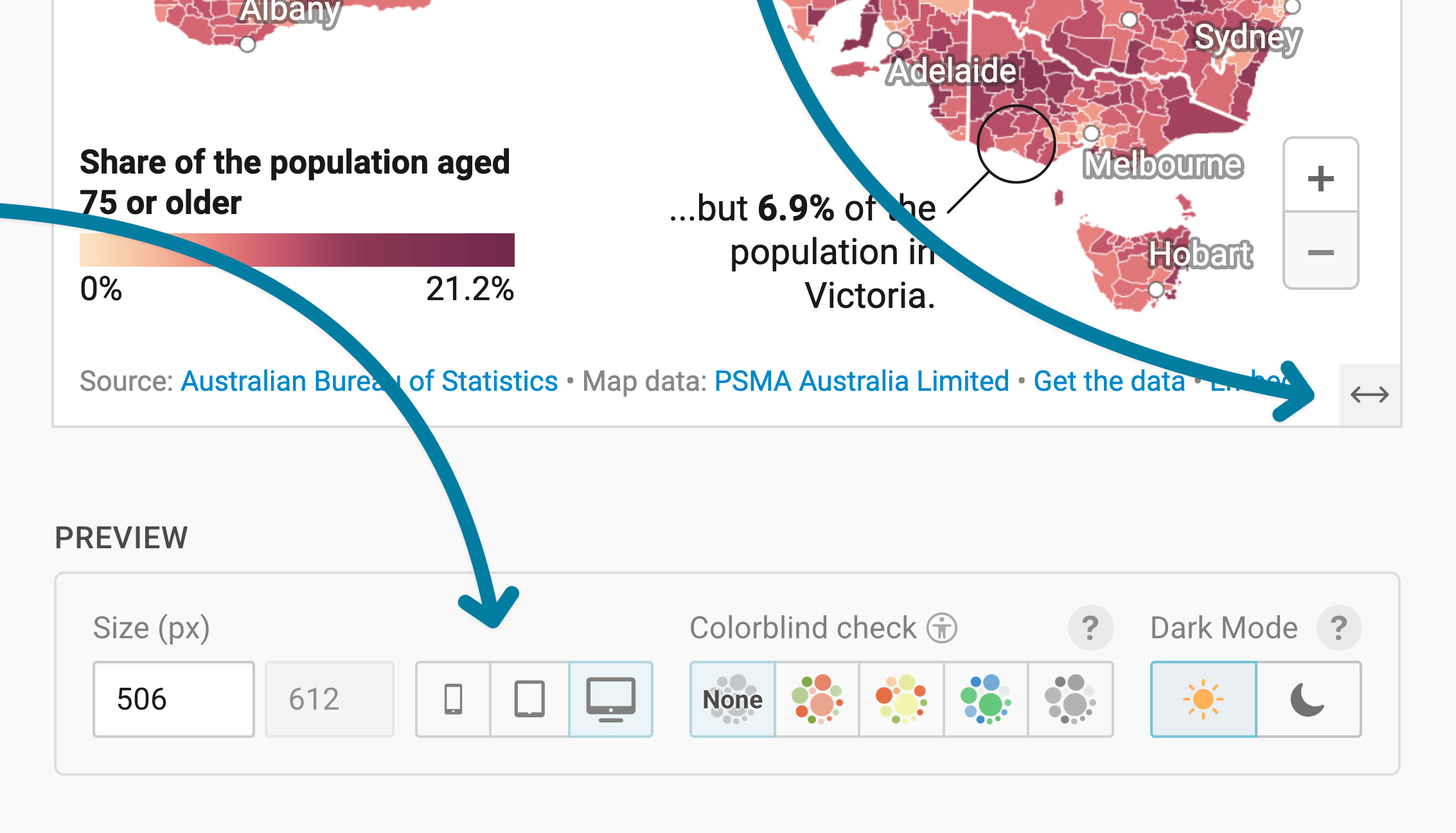
In any tab of step 3: Visualize, you can click, hold, and drag the arrow in the lower right corner to scale the map window or manually determine the dimensions of the map by entering values in the boxes below the map (Size).
We recommend checking what the map looks like on different screen sizes multiple times while designing it, by clicking on the little icons (mobile, tablet, and computer) below the map.
Learn more about changing the width and height of your map.
Refining your map
Let's continue with the Refine tab. Here, we see five panels: Colors, Patterns, Legend, Map extras, and Appearance.
Changing the colors
With the Colors panel, you can decide which colors the regions should have on your map. If you imported multiple columns, you can choose which one you want to visualize on your map at the top.
If you imported numerical values (e.g. percentages or population numbers), you'll see these options:
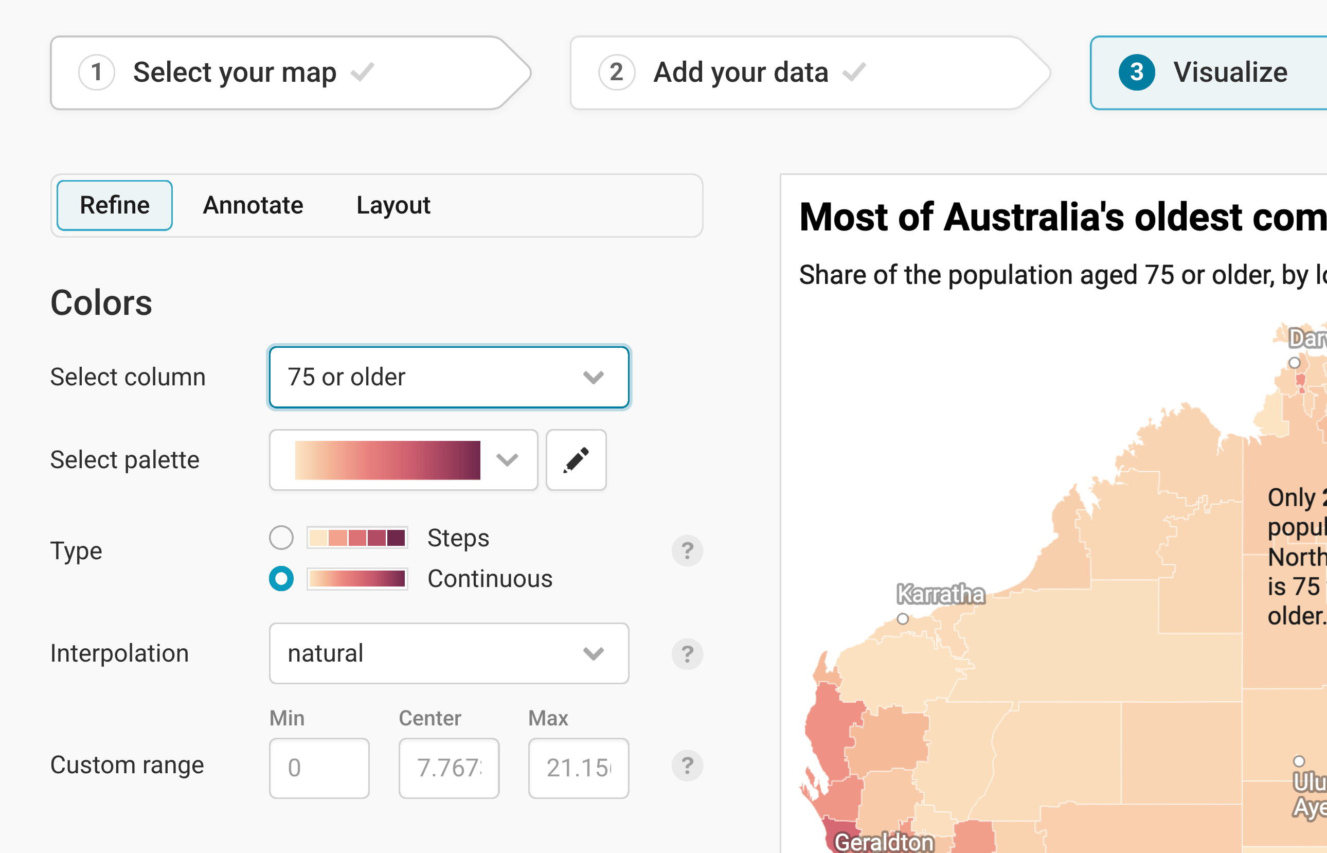
Here are the options you have:
- Select column lets you choose which of your uploaded columns you want to assign colors to in your map. Numerical columns (like our "75 or older" column) will be shown by default with a gradient. Text columns will be shown with different hues (red, yellow, blue, etc.).
- Select palette gives you a few gradients to choose from. We picked a yellow-to-red gradient instead of the default yellow-green-blue one. Click on the pen symbol next to the gradient to change the colors within a gradient. Learn more about changing your color palette.
- Type: You can decide between steps (where each color covers a range, e.g. yellow covers 5-10%), or a continuous gradient. Learn more about when to use which type on our blog, or learn how to customize stepped color scales in this Academy article.
- Interpolation: Datawrapper uses a linear interpolation by default. For our map, we chose a natural one, to bring more focus on higher values. Learn more about which interpolation to use.
- Custom range: Datawrapper automatically maps your values between the lowest and the highest number, without a center value. You can change this and enter your own values here. If you have both positive and negative values, we recommend setting "0" as a center value.
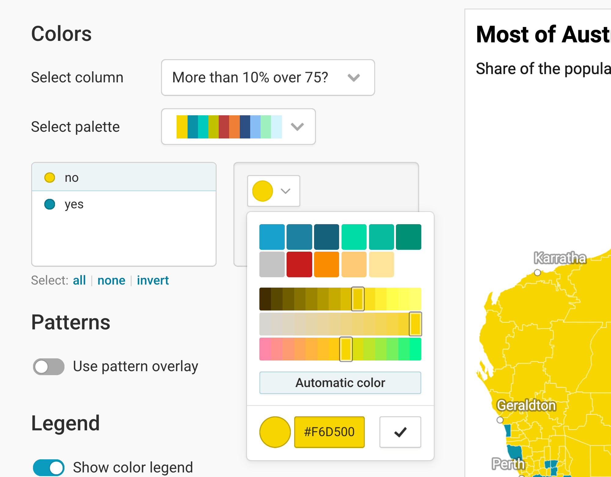
If you choose a text column, you can assign colors to categories (e.g. "yes"/"no" or "Republican"/"Democrat"/"Independent"). Click on them and then on the color swatch to change their colors:
Adding patterns
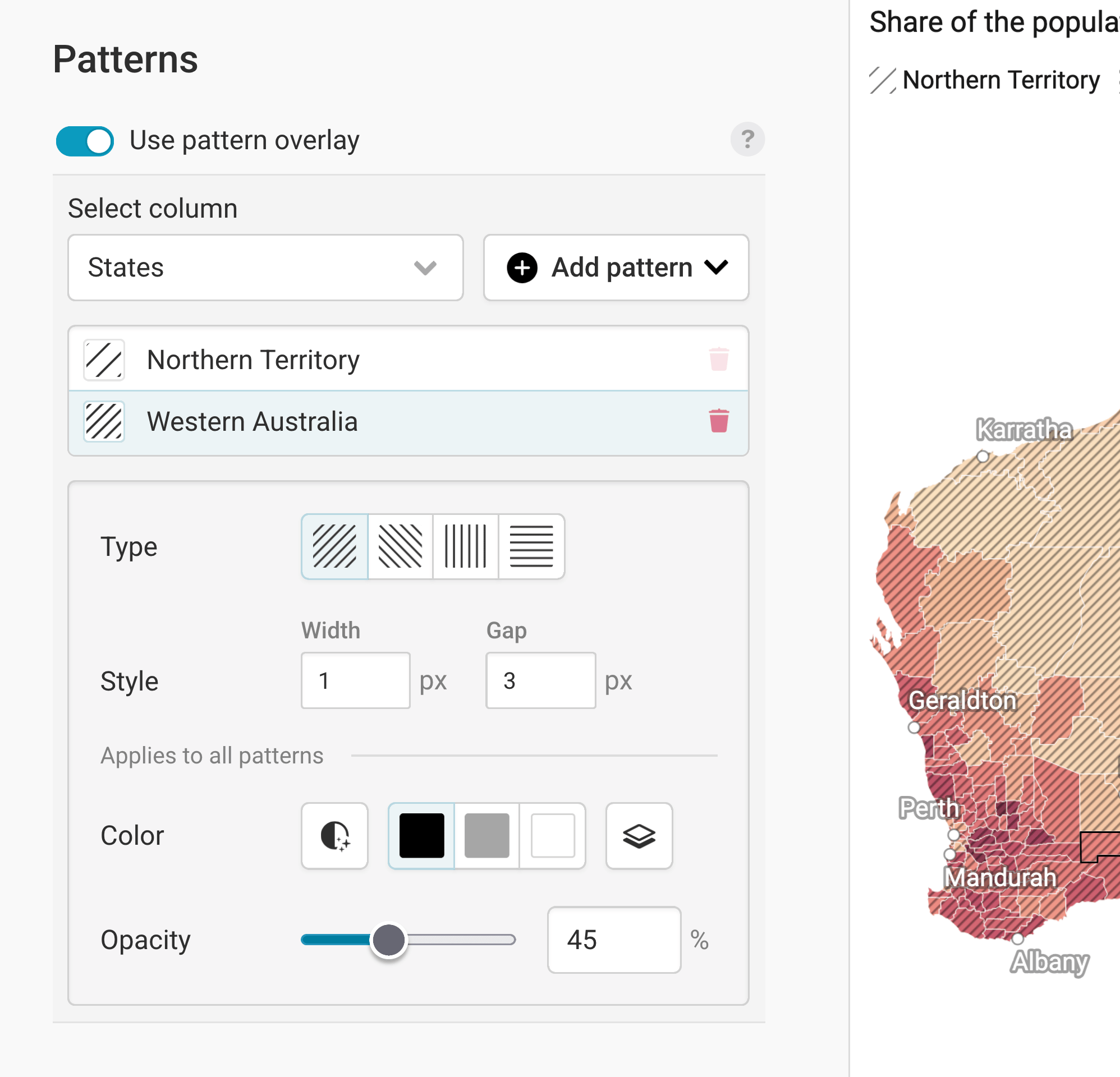
To add some additional information to your regions, you can show different patterns on them. Learn more about adding a pattern overlay to choropleth maps.
Customizing the legend(s)
Now that you settled on some nice colors (and maybe a pattern), let's make sure your audience can make sense of them. That's what a legend is for.
By default, Datawrapper shows a legend for your colors. If you add a pattern, Datawrapper will also automatically show a legend for that pattern. You can customize both in the Legend panel.
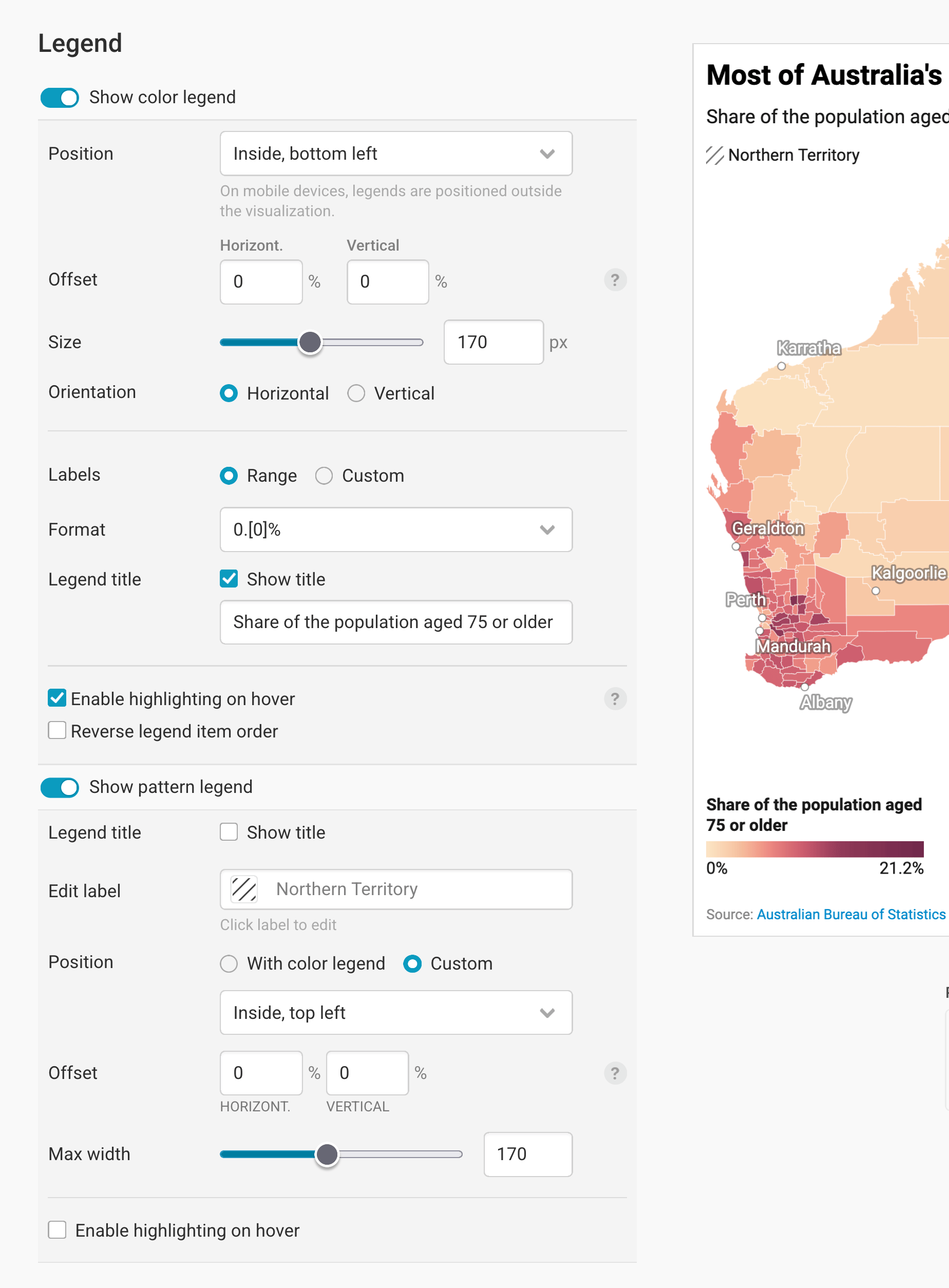
Learn more about customizing your color legend, or learn more about adding a legend for your pattern overlay.
Adding map extras
Next up, we can add extras to our map: a zoom and an inset map.
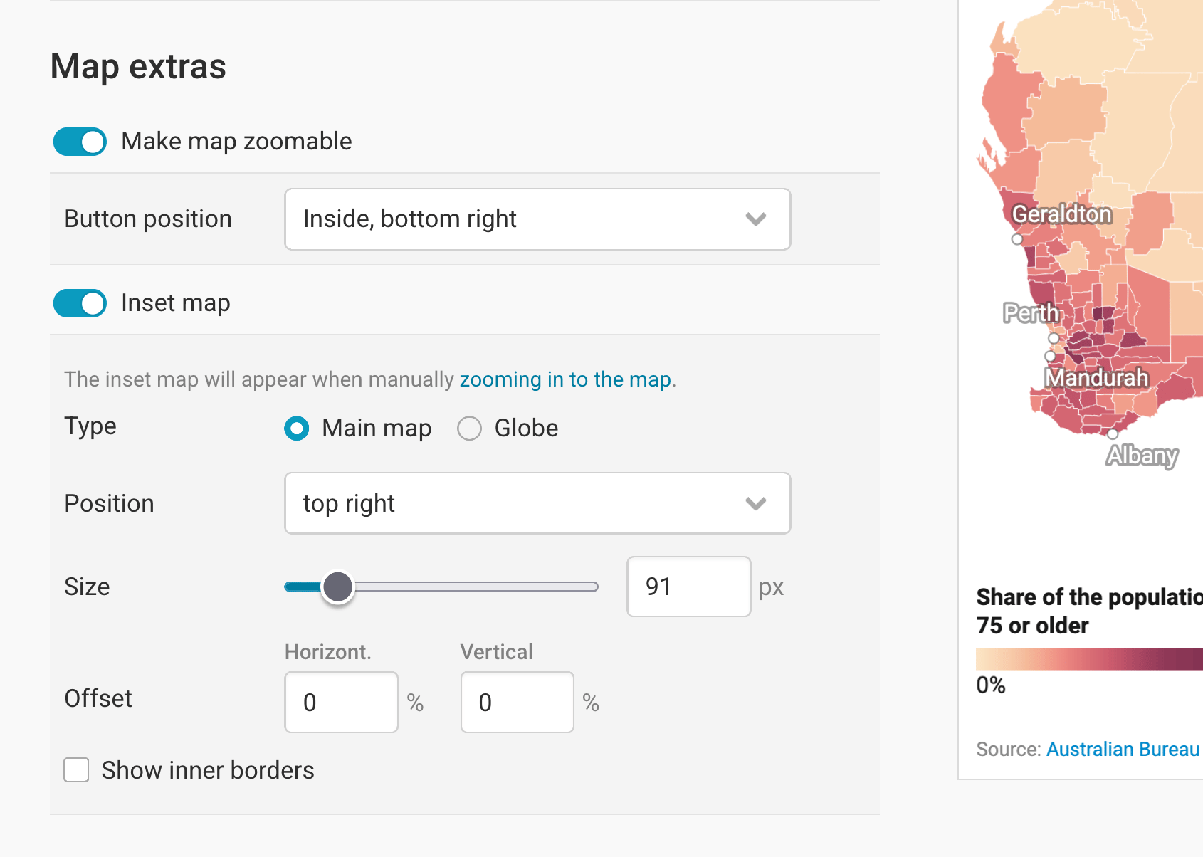
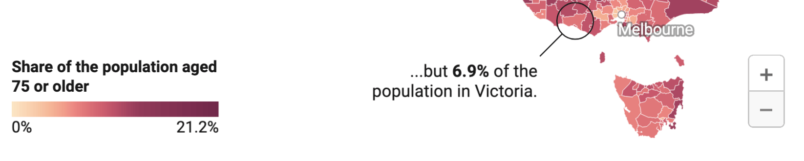
Make map zoomable makes...well, the map zoomable. You will see that this succeeded if your map gets a gray minus and plus button. You can define in which map corner the zoom buttons show up with Button position. Here, the button is in the bottom right:
Adding an inset map means adding a little map to your map that shows more context. You can choose between two types:
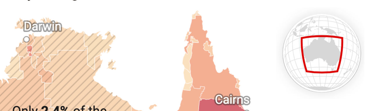
Globe: A good option if your audience might not immediately know where a country is located. (Hopefully Australia doesn't fall into that category, so a globe isn't necessary here.)
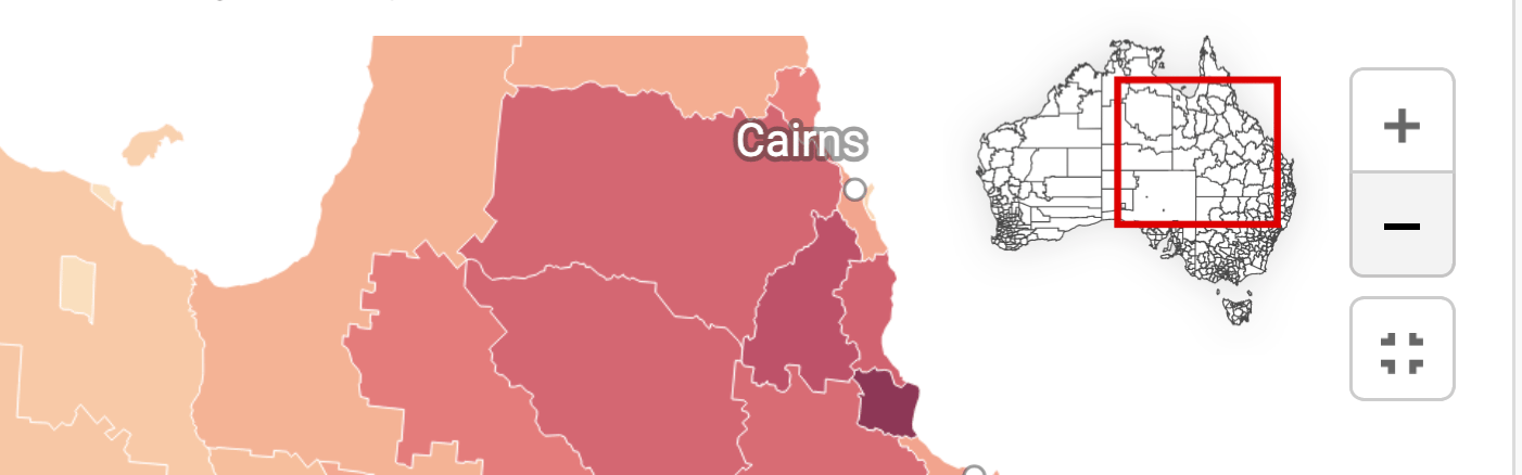
Main map: Useful when you're hiding certain map regions (learn more). It also works well alongside a zoom button: When readers zoom in, the inset appears and helps them keep track of where they are:
You can also choose the Position and Size of the inset map, and can decide how much it should move away from the map edges (in percentage of the whole map width and height).
Show inner borders shows the region borders of your map – in our case, the Local Government Areas (LGA):
Changing the appearance
In the Appearance panel, you can decide what your map looks like within the available space:
Map view: By default, the Full map is shown. Choose Crop to data to zoom into all regions for which you uploaded data. You'll get the extra option to hide the regions without data, too (learn more).
Additional padding moves the map inwards, away from the map edges. This can be useful if you need more space for your map extras or legend(s) (see above) or annotations (see below).
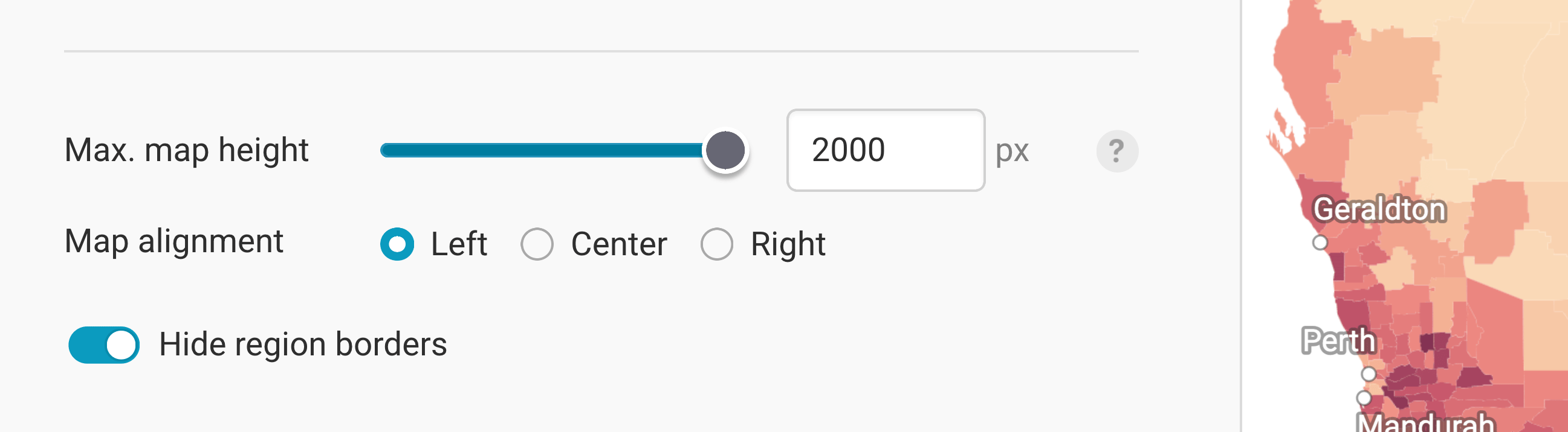
Max. map height: By default, maps will resize to fit the full width of, for example, the article where you embedded the map. But for tall, narrow maps like Chile, you may want to set a maximum height to avoid all that scrolling:
Map alignment: If you add a maximum map height and hence add extra whitespace to your map, you can choose to move your map to the left or right. Again, this can be useful to have more space for map extras, the legend(s), or annotations.
Hide region borders: This removes the white outlines around each region. The downside is that it becomes harder to tell regions apart, particularly when they share similar values. The upside is a cleaner map where borders don't get in the way of labels, patterns, and annotations.
These are all the settings you can find in the Refine tab. Let's move on to the Annotate tab:
Annotating your map
Adding a title and source
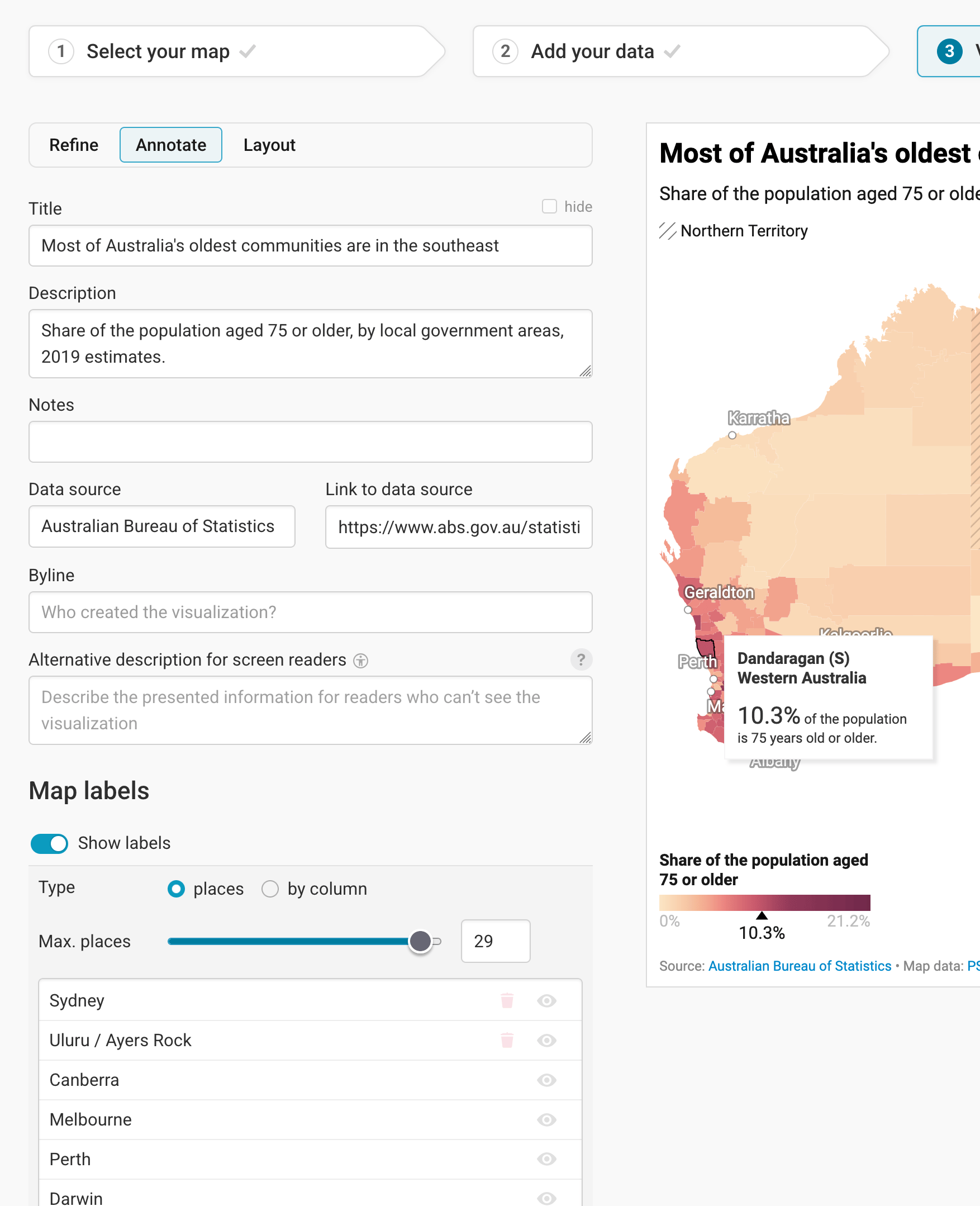
In the Annotate tab, you're first asked to give your visualization a title, description, notes, source, byline, and an alternative description for screen readers. You can find a detailed explanation of all these Annotate options here.
Adding map labels
Then there are three panels left: map labels, text annotations, and tooltips.
Map labels show the names of regions and cities directly on the map. Turn on Show labels, choose with Max. places how many labels should appear at most, and drag the places in the list to decide which ones are the most important. You can also search for more places to add. In our map, we show city names like Perth and Sydney.
To learn more, visit our article How to add map labels.
Adding text annotations
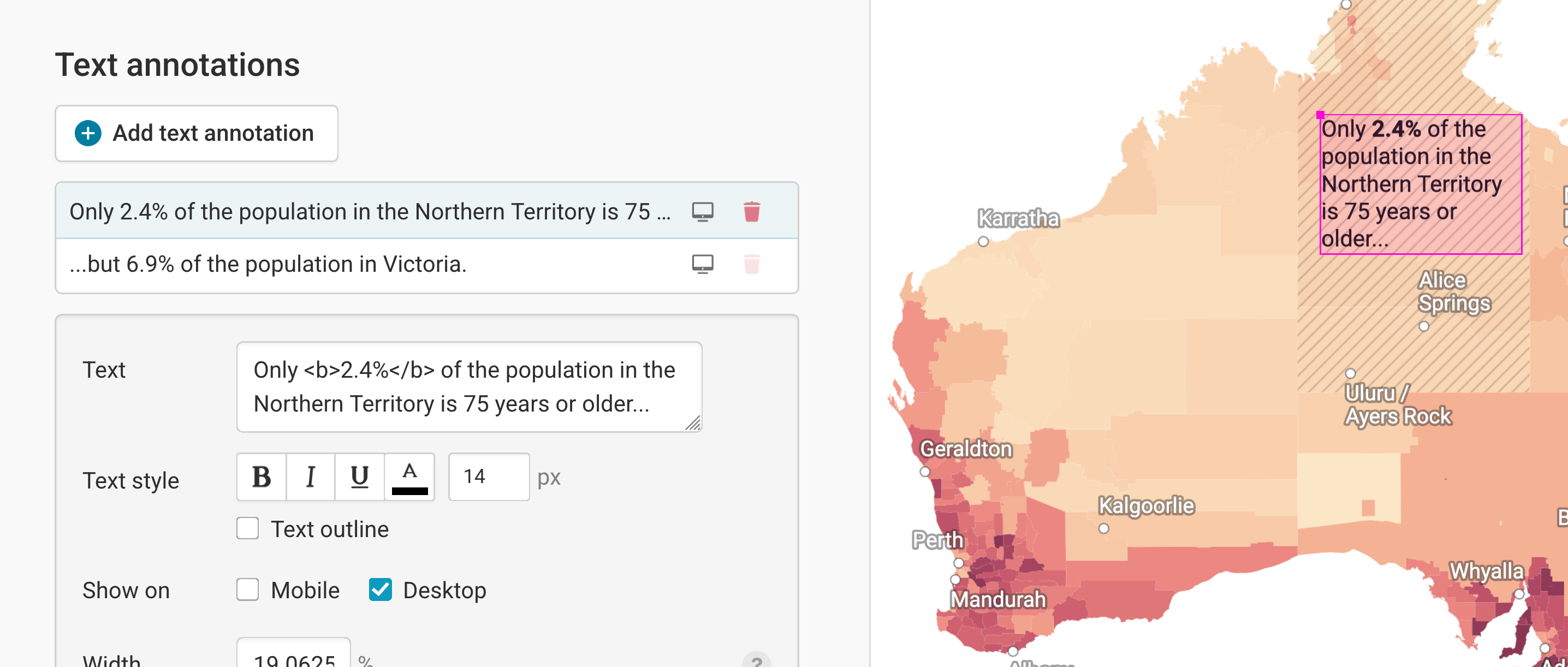
In our map, the text annotations explain the difference between the Northern Territory and Victoria. Learn more about how to create text annotations.
Creating tooltips
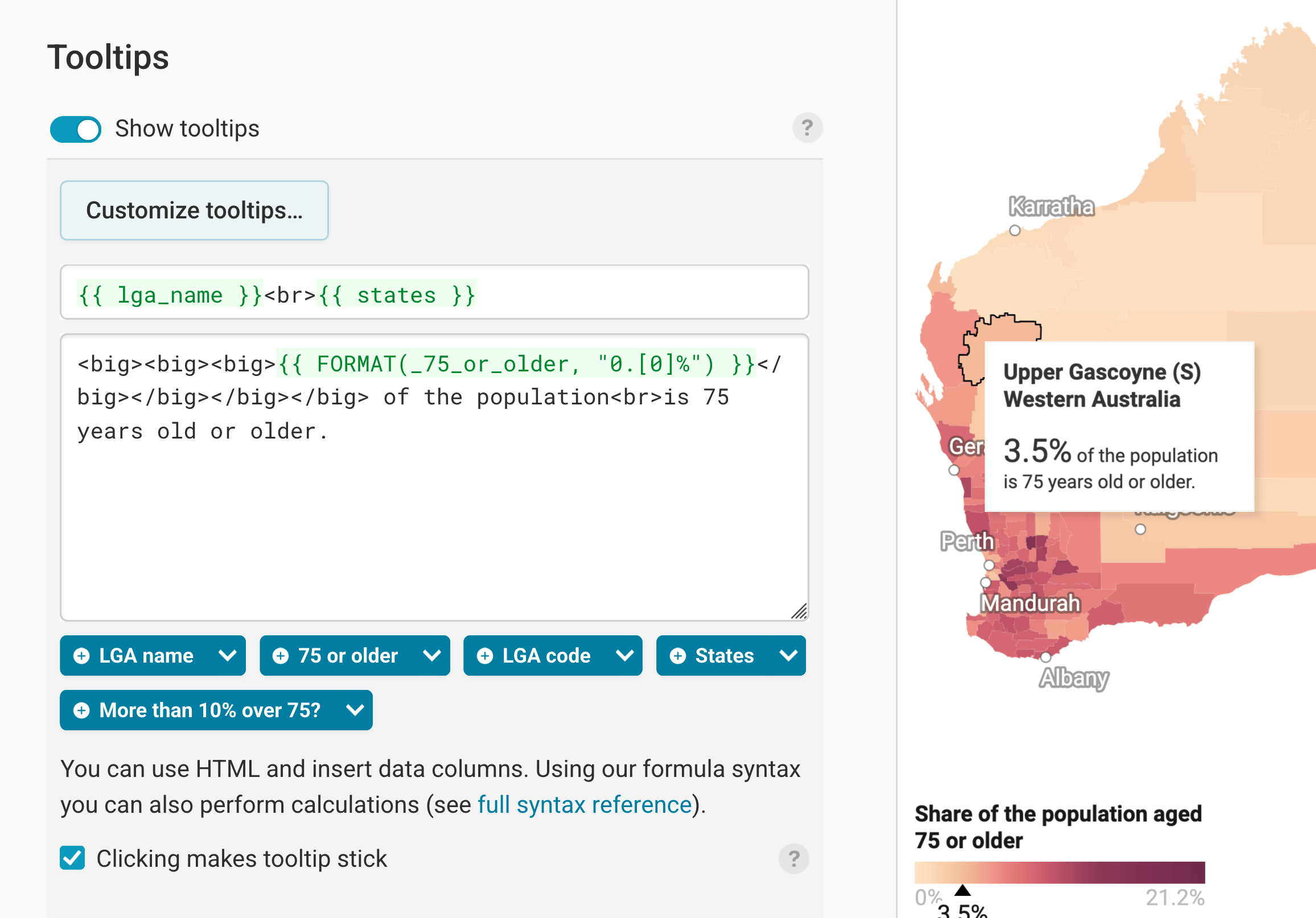
Finally, you can add tooltips. They're great to let your readers explore the map, see the underlying value of each region, and to add context information.
If you tick Clicking makes tooltip stick, the tooltip stays open when readers click on a region, so they can read it in peace.
Learn how to create them in our article How to create tooltips, and learn how to customize them.
Publishing your map
After annotating your map, only one tab is left in step 3: Visualize: the Layout tab. You can find all Layout settings explained in this Academy article.
In step 4: Publish & Embed, you can first publish your map and then decide how it gets to your readers. We recommend pasting the embed code into your website or CMS, but you can also share the map's URL. Learn more about both options here. To use your map somewhere else, download it as a PNG (on any plan) or as an SVG or PDF (on paid plans). See what each plan includes on our pricing page.
And that's it! You've successfully created and customized a choropleth map.