How to create an area chart
- Free
- Pro
- Business
- Enterprise
(Stacked) Area charts are great to show how a total and its shares developed over time. Think of it as a combination of a line chart (change over time) and a column chart (distributions & comparisons). If you're not sure if an area chart is the best choice for your data, visit our article What to consider when creating area charts.
This article explains how to create and customize the following area chart. The dataset we will be using takes a closer look at carbon emissions between 1850 and 2024.

Preparing your data
Formatting your data
To create an area chart, your dataset needs to be structured like so:
- One header row containing descriptive labels ("Year", "Liquid fuel", etc.)
- One column with dates or timestamps. This will define the horizontal axis. In our case, we plot years along the horizontal axis.
- At least one column containing numeric values. The values in these columns will define the height of the areas for each year.
The following table shows part of the data we used to create the chart at the top of the page:
| Year | Solid fuel | Liquid fuel | Gas fuel | Cement production | Gas flaring | Other |
| 1920 | 855000000 | 98500000 | 11400000 | 2500000 | 0 | 600000 |
| 1921 | 729300000 | 108400000 | 9600000 | 2400000 | 0 | 500000 |
| 1922 | 756900000 | 119600000 | 10900000 | 2900000 | 0 | 700000 |
| 1923 | 859600000 | 132500000 | 14300000 | 3400000 | 0 | 700000 |
| 1924 | 861300000 | 132100000 | 16300000 | 3700000 | 0 | 700000 |
| 1925 | 860700000 | 138000000 | 17400000 | 3900000 | 0 | 800000 |
| 1926 | 841700000 | 138200000 | 18900000 | 4000000 | 0 | 800000 |
Uploading your data
Once you have prepared your data, create a new chart in Datawrapper. You can do so by going to our homepage and clicking on Start creating. In step 1: Upload, you can copy & paste your dataset, upload it as a .csv or Excel file, or connect to a Google Sheet.
If you want to create the chart at the top of this Docs article, click on Select a sample dataset at the bottom of the page and choose the dataset Global CO2 Emissions. After importing the data, the text field on the right will look something like this:
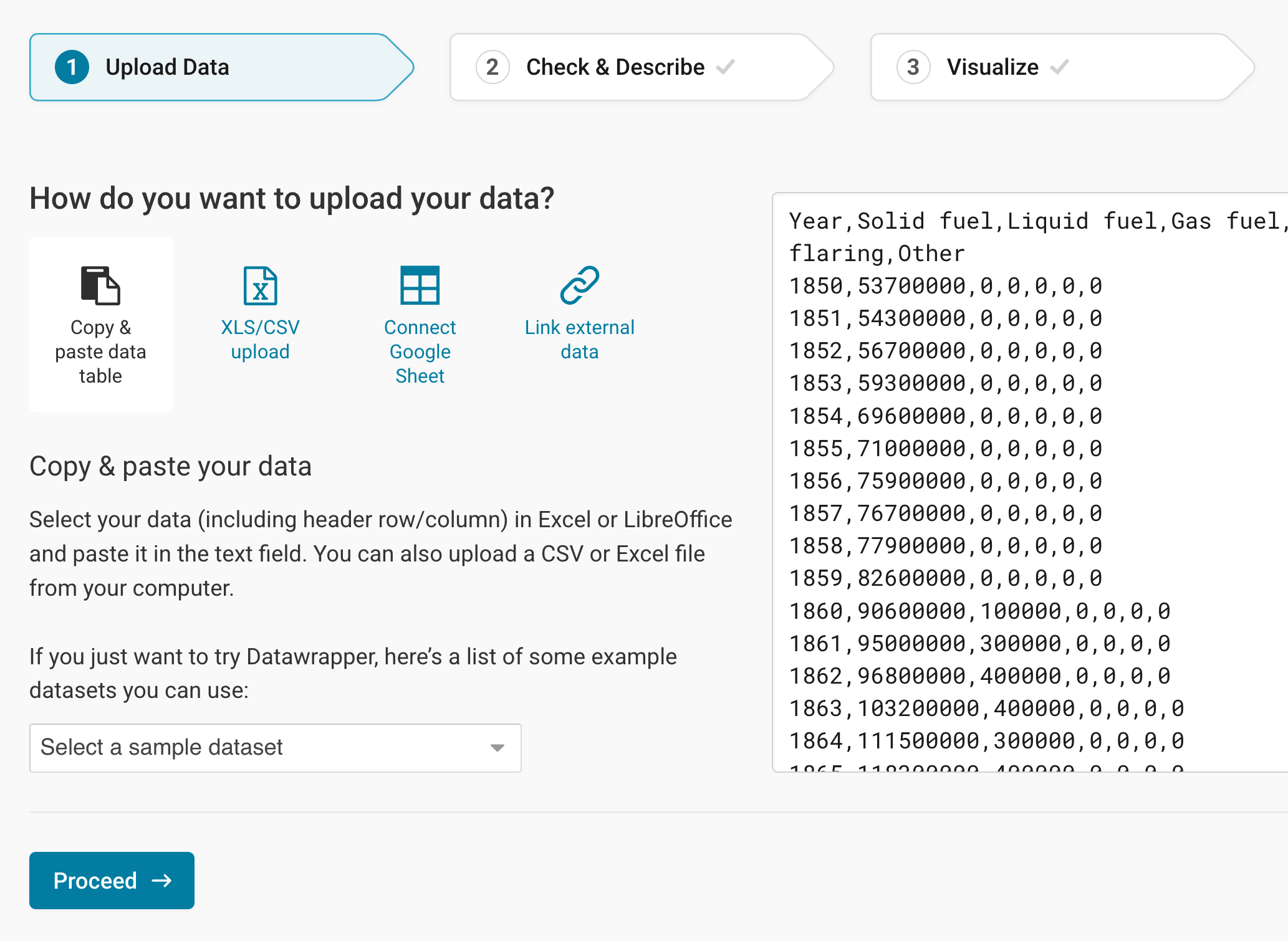
Click Proceed at the bottom left to go to the next step.
Checking data and units
In step 2: Check & Describe, you can check if your dataset was imported correctly and make changes to it, if necessary.
You can see that Datawrapper correctly recognized your numbers as numbers (and not as text or dates) because they are colored in blue and are right-aligned. Learn more about Datawrapper's automatic recognition of data formats.
If you did not upload a header row, untick First row as label to avoid losing your first row of data.
To add a unit (like km/h, kg, inch, $, etc.) to your numbers, click on a column header and then add the unit of your choice to the Prepend/append options on the left. You can learn more about adding units to numbers here.
Click on Proceed at the bottom left to go to step 3: Visualize.
Choosing an area chart
In step 3: Visualize, click on the Area chart symbol in the grid of available chart types:
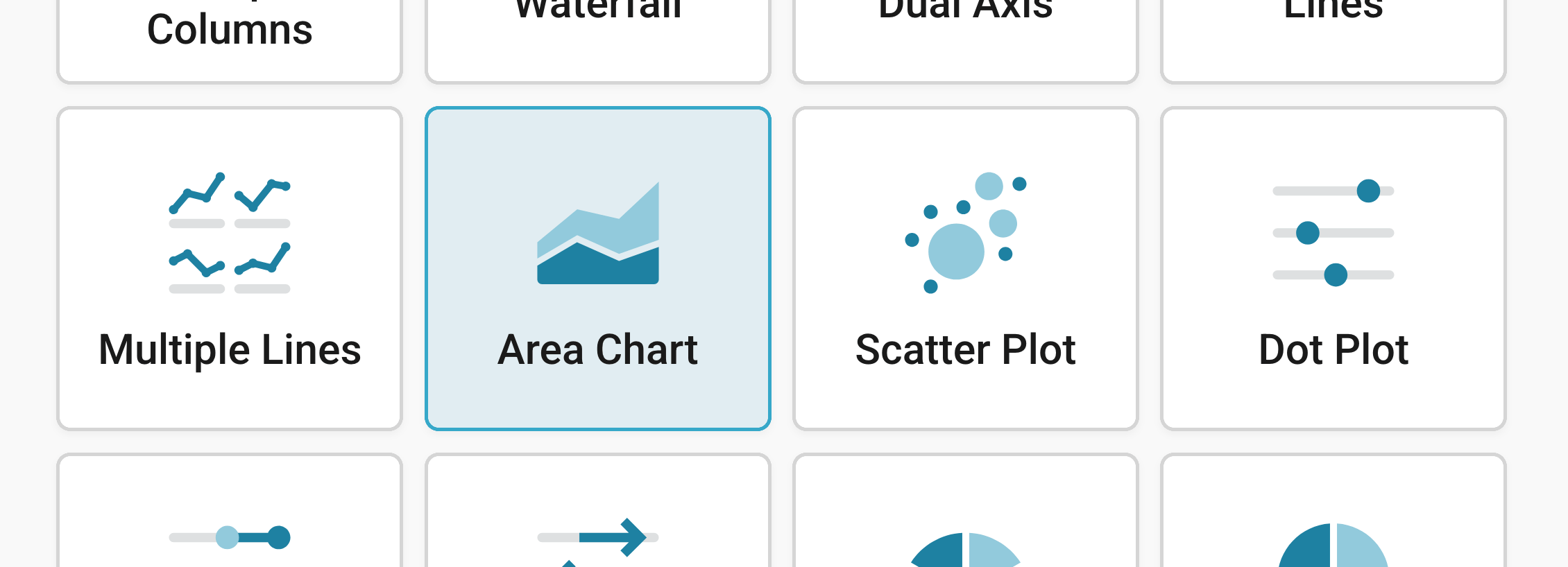
You will now see an area chart, without a title, descriptions or customized colors.
Next, we want to further refine and annotate this chart. Besides Chart type, you'll notice three more tabs in this step: Refine, Annotate, and Layout.
Resizing
In any tab of step 3: Visualize, you can click, hold, and drag the arrow in the lower right corner to scale the chart window or manually determine the dimensions of the chart by entering values in the boxes below the chart (Size).
We recommend checking what the chart looks like on different screen sizes multiple times while designing it, by clicking on the little icons (mobile, tablet, and computer) below the chart.
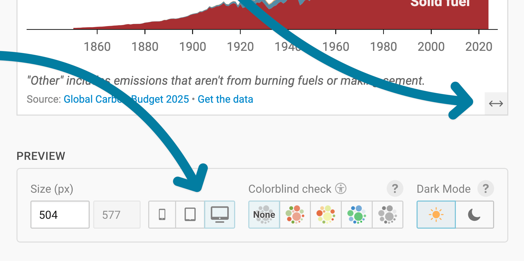
Learn more about changing the width and height of your chart in this article.
Refining your chart
Changing the horizontal axis
First, the horizontal axis. For this axis, you should select the column in your data that has the time data (dates, years, time stamps, etc.), if it's not already selected by default. We choose the column "Year" for our horizontal axis.
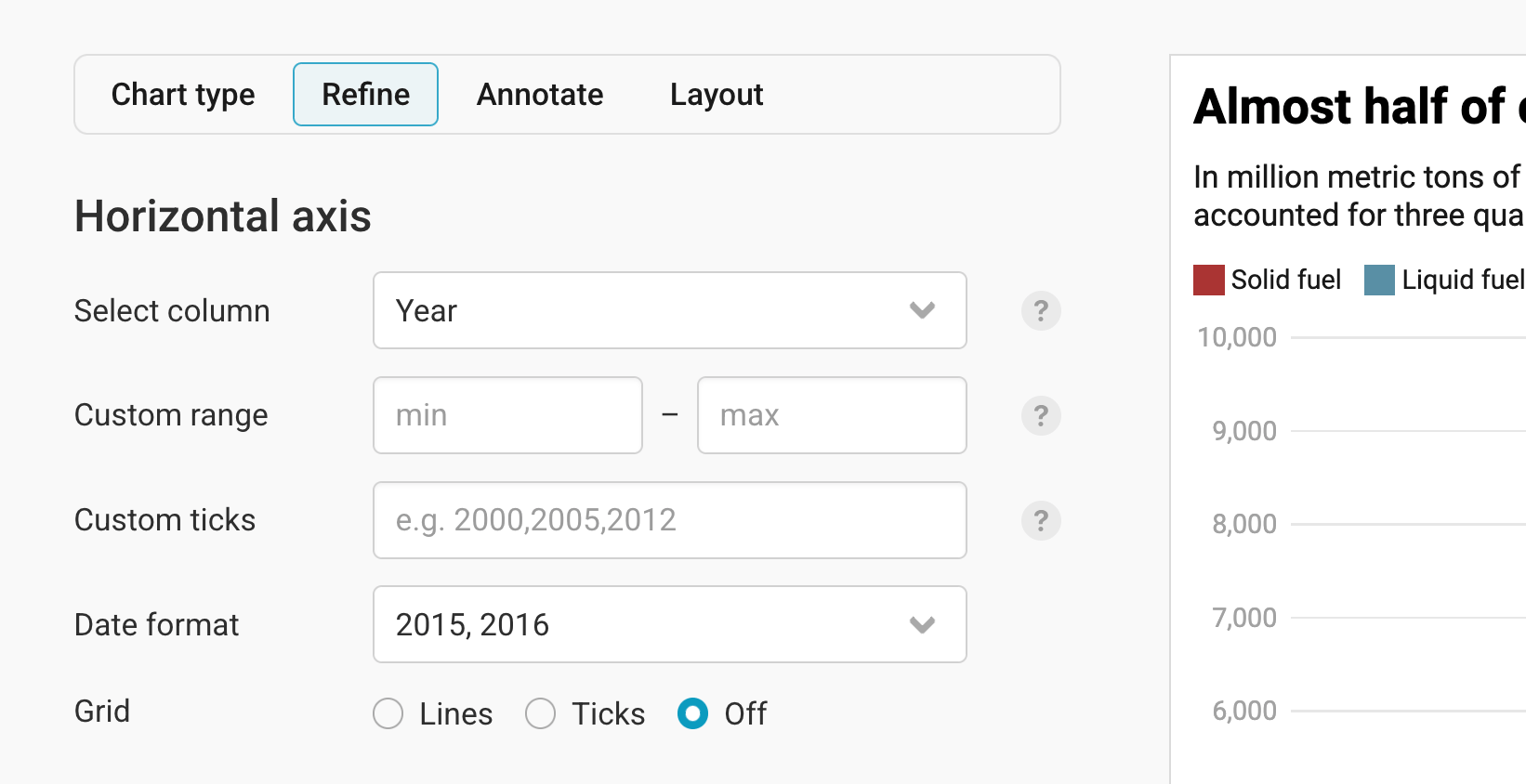
These are the other settings in this panel:
- Custom range: Here you can show a time range other than the one that is automatically displayed. By default, the horizontal axis spans from the earliest to the latest date – but you can decide to cut off data points or extend your axis here. For example, you can decide to only show data points between 2010 and 2018, even if the data goes from 2000 to 2022.
- Custom ticks: Here you can decide on the number of ticks you want to see. If you type in "2000, 2005, 2006", only three gridlines and grid labels will appear on the horizontal axis.
- Date format: Here you can decide which kind of ticks you want to see. We have yearly data, and the date format "2015, 2016" works well for us. Datawrapper won't display ticks for each of the years, because the space is too limited to do so. Learn more about displaying dates in this article.
- Grid: Here you have three options: Lines (to see the vertical gridlines going from the top to the bottom), Ticks (to only have short lines below the x-axis), and Off (to not show the gridlines at all). Whichever option you choose depends on your personal preference and how many ticks you show on the chart.
Here's how our horizontal axis looks in the final chart with the settings you can see in the last screenshot:

Changing the vertical axis
The settings for the vertical axis are similar to those for the horizontal axis:
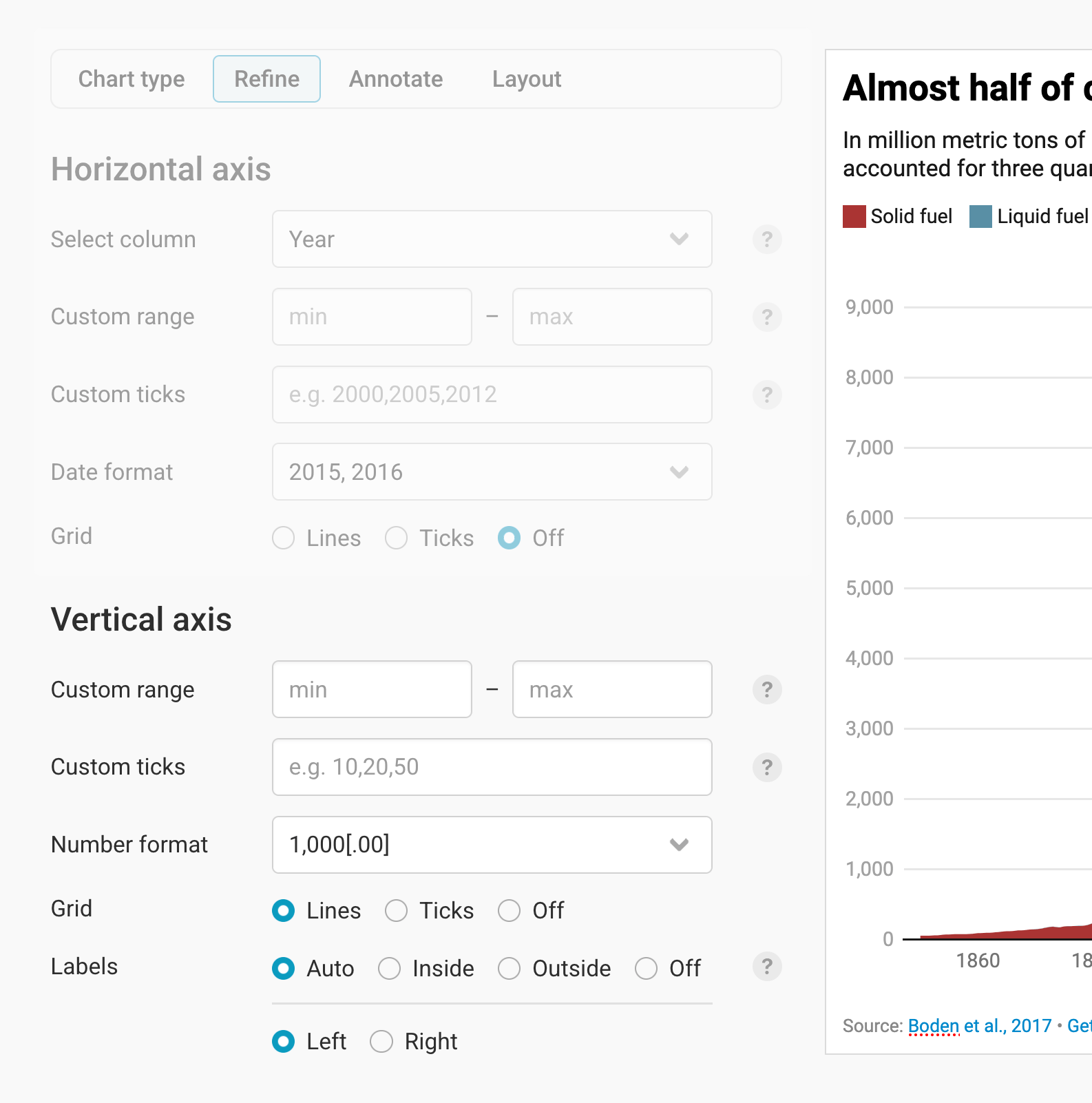
- Custom range lets you define the lowest and highest value on the axis. By default, the vertical axis spans from the lowest to the highest number – but you can decide to cut off data points or extend your axis.
- Custom ticks: Decide on the number of ticks you want to see. If you type in "5000,7000", only two gridlines and grid labels will appear.
- Number format: Decide how your values show up in the grid labels. You can learn more about number formats in this Docs article.
- Grid: This is the same as on the horizontal axis. Here, too, you have three options: Lines (to see the horizontal gridlines going from left to right), Ticks (to only have short lines next to the y-axis), and Off (to not show the gridlines at all).
- Labels: Define how gridline labels are positioned: Inside places the labels on the gridlines, Outside places them next to the gridlines. Choose Off if you don't want to show any labels at all. With Auto, the position is automatically adjusted to the limited space available on mobile. You can also choose if you want the y-axis to show up on the left or the right side of the chart.
Styling your areas
The most important setting of this panel is choosing colors for your areas.
You can choose one color for all your areas (click on the color panel next to Base color to change the default color) – all areas will then appear in this color and its shades.
You can also adjust the colors manually for each area. To do so, click on Set colors next to the base color:
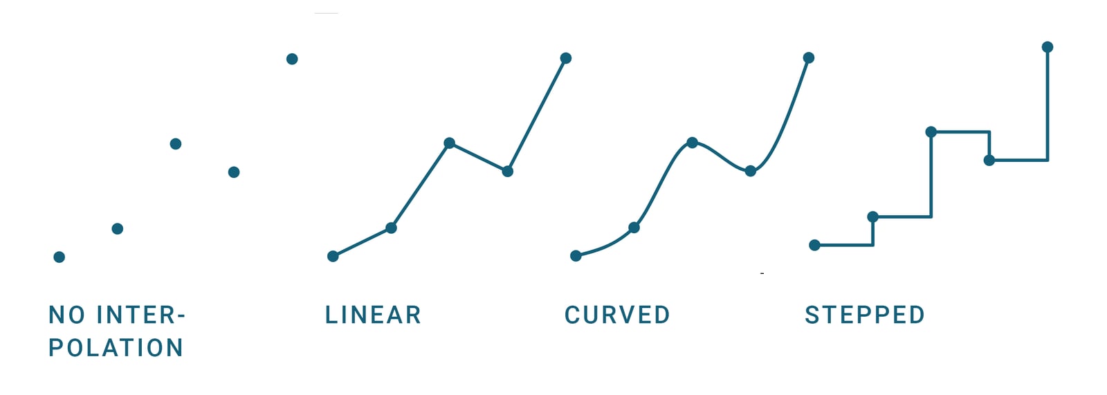
Below the color settings, you can change the opacity of your areas (having an effect on how much the gridlines shine through) and interpolation. Interpolation refers to how Datawrapper draws lines between the available data points. To read more about when to choose which interpolation, visit our blog post.
There are two more options here:
- Sort areas: Decide if you want to keep the order in which you uploaded your columns in, or show the smallest first (meaning, smaller areas on the bottom of the chart) or the largest first (bigger areas are on the bottom).
- Stack areas: Stacked means that all areas are on top of each other. If you turn this off, the areas will overlap instead. This is harder to read and only a great option in a few cases, so stacked areas are the default in Datawrapper. You can also choose to stack areas to 100% – so that your audience can compare the share of your categories – or to separate the areas with lines in a certain line color. Here's what a 100% area chart looks like:
Changing the legend and tooltips
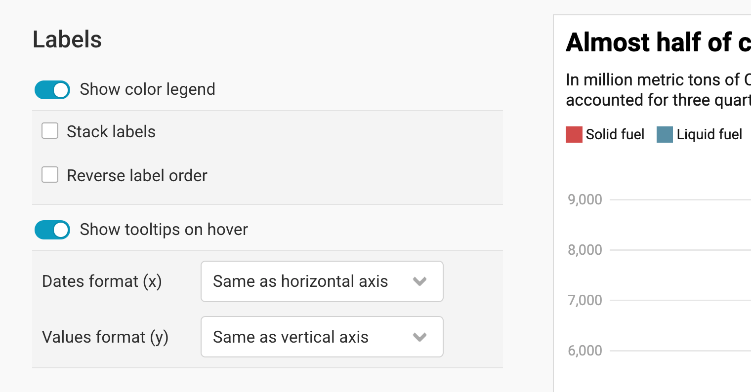
In this fourth panel, you can customize your color legend and tooltips.
By default, Show color legend is turned on. Think twice before you turn it off, since there's no other built-in way to show your audience what each area means.
Stack labels means that your color legend items show up below each other instead of next to each other. This can be useful if you only have two or three areas with very long color legend labels. Here's what this looks like:
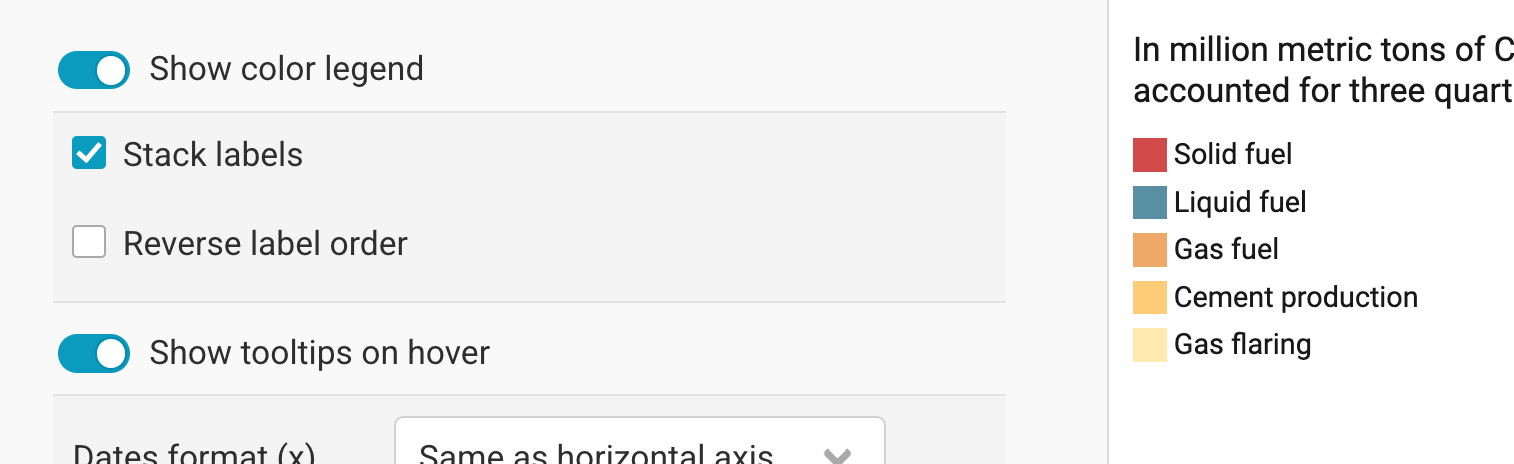
Reverse label order does exactly that: The first item in your color key becomes the last one, and the other way around.
You can also choose whether your audience should see tooltips when they hover over an area in the embedded version. If you turn tooltips on, you can change the date format and the number format to be different from the horizontal and vertical axis.
Changing the height
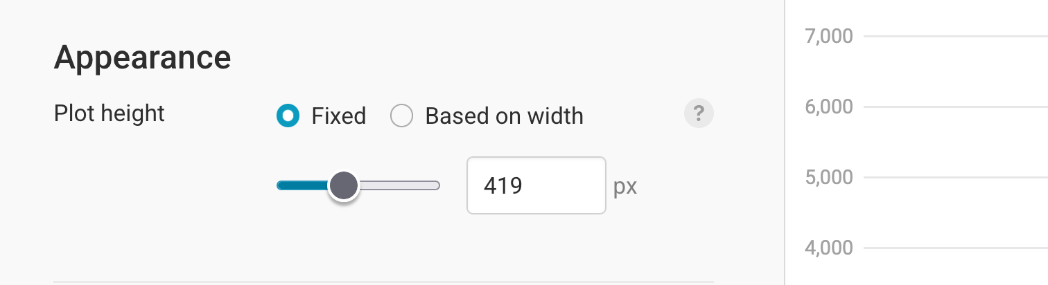
The last settings in the Refine tab let you change the plot height. You can learn more about the available options in this article.
Let's move on to the next tab, Annotate:
Annotating your chart
Adding a title and source
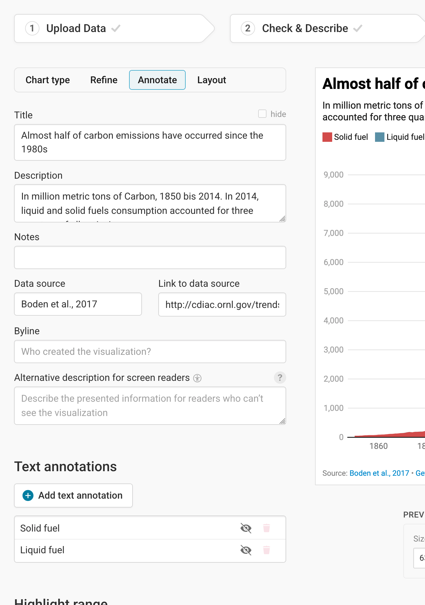
In the Annotate tab, you're first asked to give your visualization a title, description, notes, source, byline, and an alternative description for screen readers. You can find a detailed explanation of all these Annotate options here.
Adding text annotations
You can then add and customize text annotations anywhere on your area chart. Learn how to create text annotations here.
Highlighting ranges
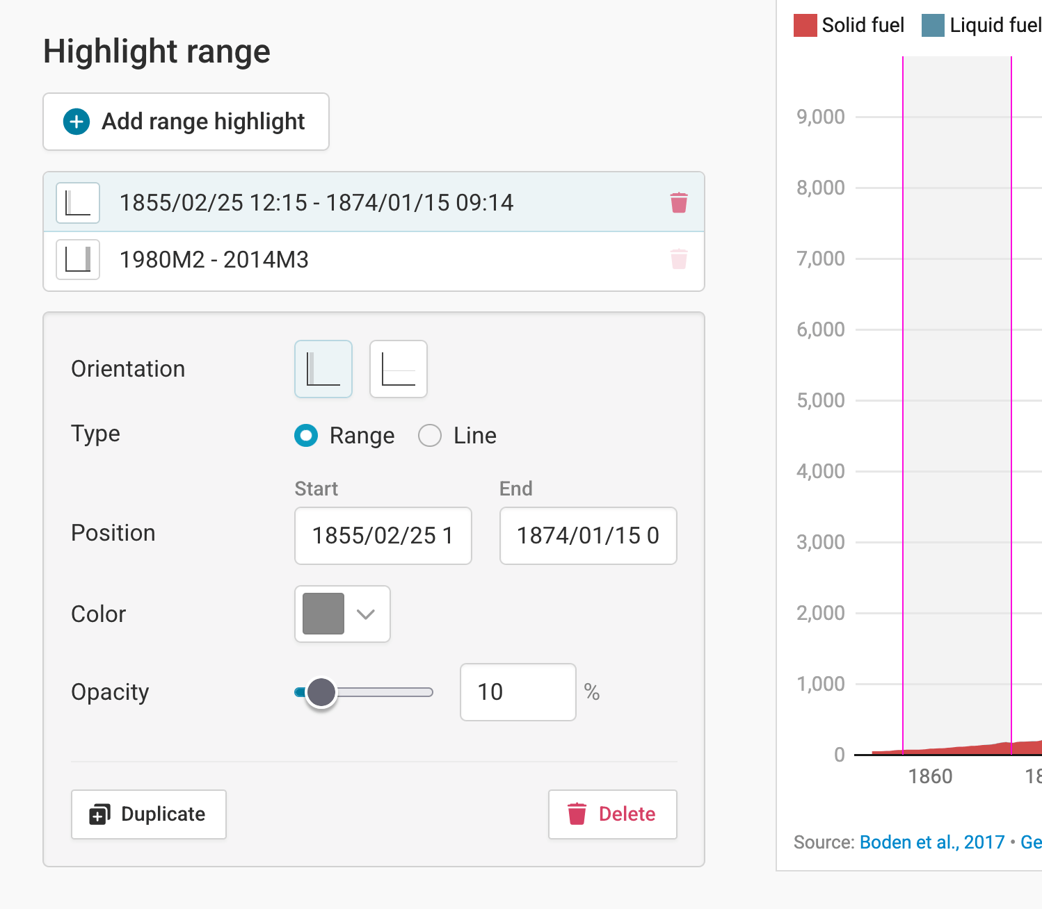
Finally, if you want to draw your reader's attention to one specific time range, the Highlight range tool is perfect. It lets you set semi-transparent colored overlays directly in your chart. To do so, click on Add range highlight. Now select a starting and ending point of the range by clicking in the chart. If you want, you can also change the opacity of the highlighted range. Here's an in-depth explanation of all the options.
Publishing your chart
After adding text to our chart, only one tab is left in step 3: Visualize: the Layout tab. You can find all Layout settings explained in this Docs article.
In step 4: Publish & Embed, you can first publish your chart and then decide how it gets to your readers. We recommend pasting the embed code into your website or CMS, but you can also share the chart's URL. Learn more about both options here. To use your chart somewhere else, download it as a PNG (on any plan) or as an SVG or PDF (on paid plans). See what each plan includes on our pricing page.
And that's it! You've successfully created and customized an area chart.