How to create a scatter plot
- Free
- Pro
- Business
- Enterprise
The scatter plot is perfect when you want to show the relationship (also called correlation) between two quantitative measures. Each dot of the chart is stands for a category (e.g. a country) and is placed on a grid according to its values for two variables. Scatter plots come from science, and many readers may find them confusing at first. Before you use one, ask yourself if it’s worth it, since some people might give up on your chart instead of reading it.
This article explains how to create and customize the following scatter plot. It shows how the GDP per capita relates to the life expectancy in selected countries:

We recommend to add hints to your readers how to read a scatter plot – for example, with annotations, or in the description. Also, remember not to confuse correlation with causation, no matter how strong your trend line appears to be.
Let's see how to create a scatter plot:
Preparing your data
Formatting your data
To create a scatter plot, our dataset should be formatted as follows. You'll need:
- One header row containing labels.
- The first column with the labels of your dots, like the country names in our data.
- At least two columns with numbers. Their values will be used as x- and y-coordinates and define the position of each dot.
The values don't have to be of the same measure. In our example, the GDP per capita is in US-Dollars, and the life expectancy is in years.
You can also add more columns: a text column to give groups of dots their own color or shape, or a number column to size your dots. In our chart, we use the continent of each country for the colors and its population for the size (more on that below).
That's what the first five rows of our data look like for the chart you can see above:
| Country | Continent | GDP per capita | Life expectancy | Population |
| Afghanistan | Asia & Oceania | 2037 | 68.8 | 42647492 |
| Albania | Europe | 18920 | 79.8 | 2791765 |
| Algeria | Africa | 15442 | 76.2 | 46814308 |
| Andorra | Europe | 65928 | 84.1 | 81938 |
| Angola | Africa | 7344 | 64.5 | 37885849 |
Uploading your data
After you have prepared your data, create a new chart in Datawrapper. You can do so by going to our homepage and clicking on Start creating. In step 1: Upload, you can copy & paste your dataset, upload it as a .csv or Excel file, or connect to a Google Sheet. It will look like this:
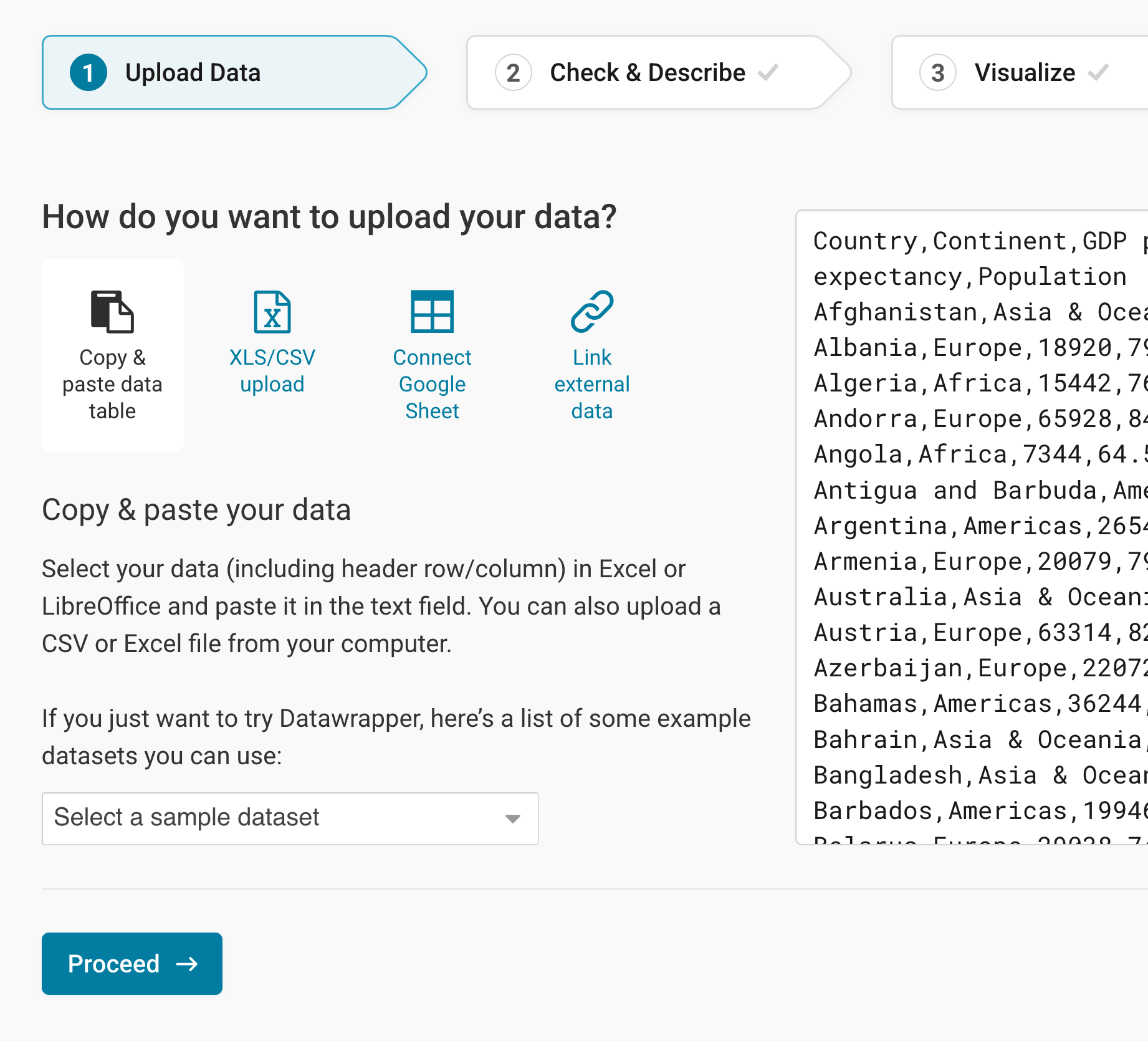
Once you're done adding your data, click on Proceed in the lower left to go to step 2: Check & Describe.
Checking data and units
In step 2: Check & Describe, you can see what the dataset looks in structured form. Make sure that the box First row as label is ticked, so that Datawrapper correctly assigns the values to the labels:
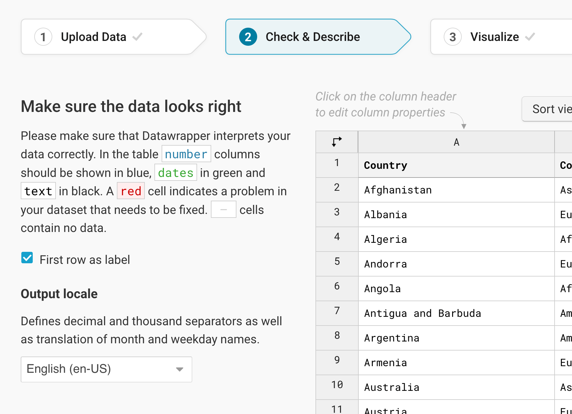
To add a unit (like km/h, kg, inch, $, etc.) to your numbers, click on a column header and then add the unit of your choice to the Prepend/append options on the left. You can learn more about adding units to numbers here.
Click on Proceed, and Datawrapper will take you to the next step.
Choosing a scatter plot
Once you're in step 3: Visualize, choose Scatter Plot from the grid of available chart types, and Datawrapper will create a first version of your chart.
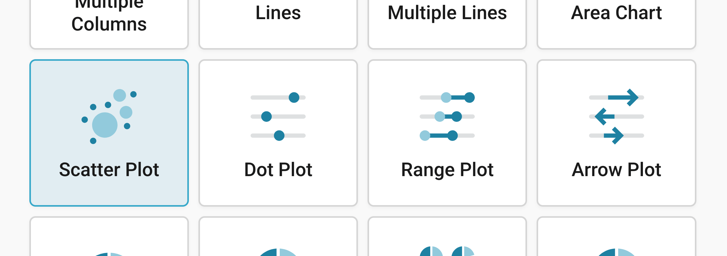
Besides Chart type, you'll notice three more tabs in step 3: Refine, Annotate, and Layout:

Resizing
In any tab of step 3: Visualize, you can click, hold, and drag the arrow in the lower right corner to scale the chart window or manually determine the dimension of the chart by entering values in the boxes below the chart (Size).
We recommend checking what the chart looks like on different screen sizes multiple times while designing it, by clicking on the little icons (mobile, tablet, and computer) below the chart.
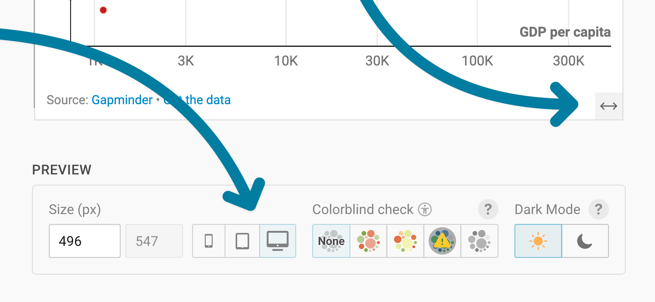
Learn more about changing the width and height of your chart in this article.
Refining your chart
Let's continue with the Refine tab. Here, we see seven panels: Horizontal axis, Vertical axis, Color, Size, Shape, Trend line, and Appearance.
Changing the axes

The Horizontal axis and Vertical axis panels have the same settings. They let you decide which data your chart shows, and how:
- Select column: lets you choose the column you want to show on this axis. In our chart, that's "GDP per capita" for the horizontal axis and "Life expectancy" for the vertical axis.
- Custom range: sets the smallest and largest value of the axis. By default, Datawrapper sets the range based on your data. If your axis should start at zero, for example, type "0" into the min field. In our chart, the horizontal axis goes up to 500,000.
- log.: turns the axis into a logarithmic scale. Log scales are harder to understand for readers, but they help to show differences between dots that are clustered at one end of the axis. We use one for the GDP per capita, since many countries have a low GDP per capita, and only a few have a very high one.
- Custom ticks: sets which values appear on the axis. If you type in "50, 100", the axis only shows ticks at 50 and 100. By default, Datawrapper decides.
- Number format: decides how the numbers on the axis look ((automatic) by default). For the GDP per capita, we chose 123k, which shows "8000" as "8k" and "1000000" as "1m". Learn more about number formats.
- Position: moves the axis to the other side of the chart. The defaults are bottom for the horizontal axis and left for the vertical axis.
- Grid: shows grid lines and axis labels (On, the default), neither of them (Off), Just lines, or Just labels.
Changing the colors
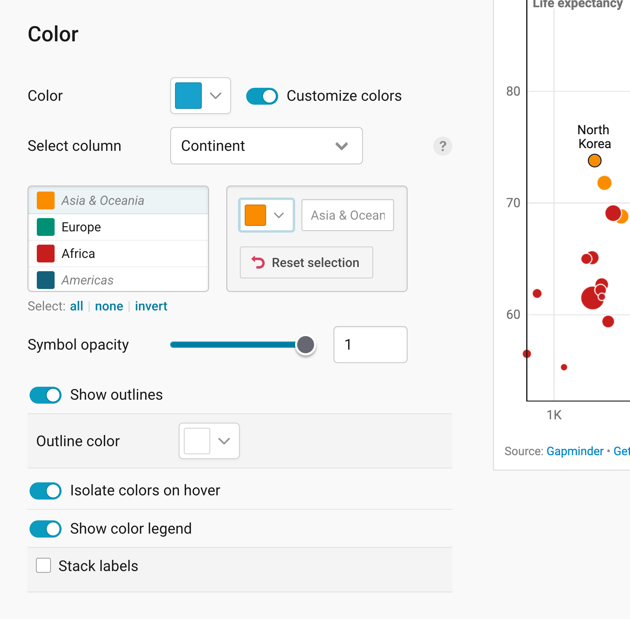
The Color panel lets you choose the colors of your dots:
- Color: sets one color for all dots.
- Customize colors: gives groups of dots their own color. Under Select column, choose a text column, like "Continent" in our chart. Then click on a group in the list and pick a new color. all, none, and invert below the list help you select many groups at once. Reset all changes undoes all your colors.
- Symbol opacity: makes your dots more transparent. The default is 1, meaning not transparent at all. Making your symbols less opaque helps when a lot of your dots overlap.
- Show outlines: adds an outline around each dot, in the Outline color of your choice. That also helps with overlapping dots. We use white outlines in our chart.
- Isolate colors on hover: lets readers highlight all dots of one color by hovering over it in the color legend or on one dot.
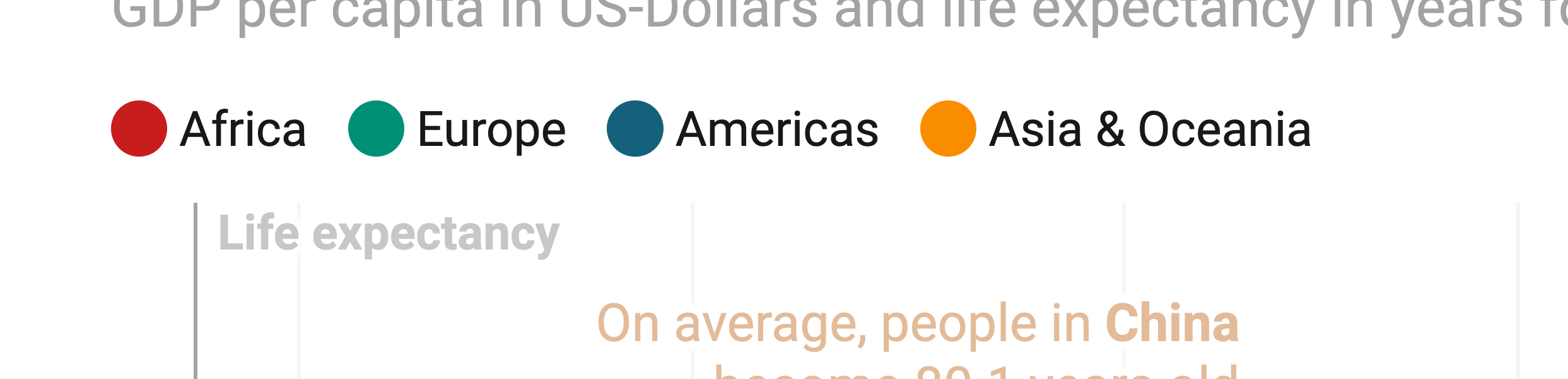
- Show color legend: shows which color stands for what, above your chart. With Stack labels, the names appear below each other instead of next to each other.
Here's what the color legend looks like in our chart:
Sizing the dots
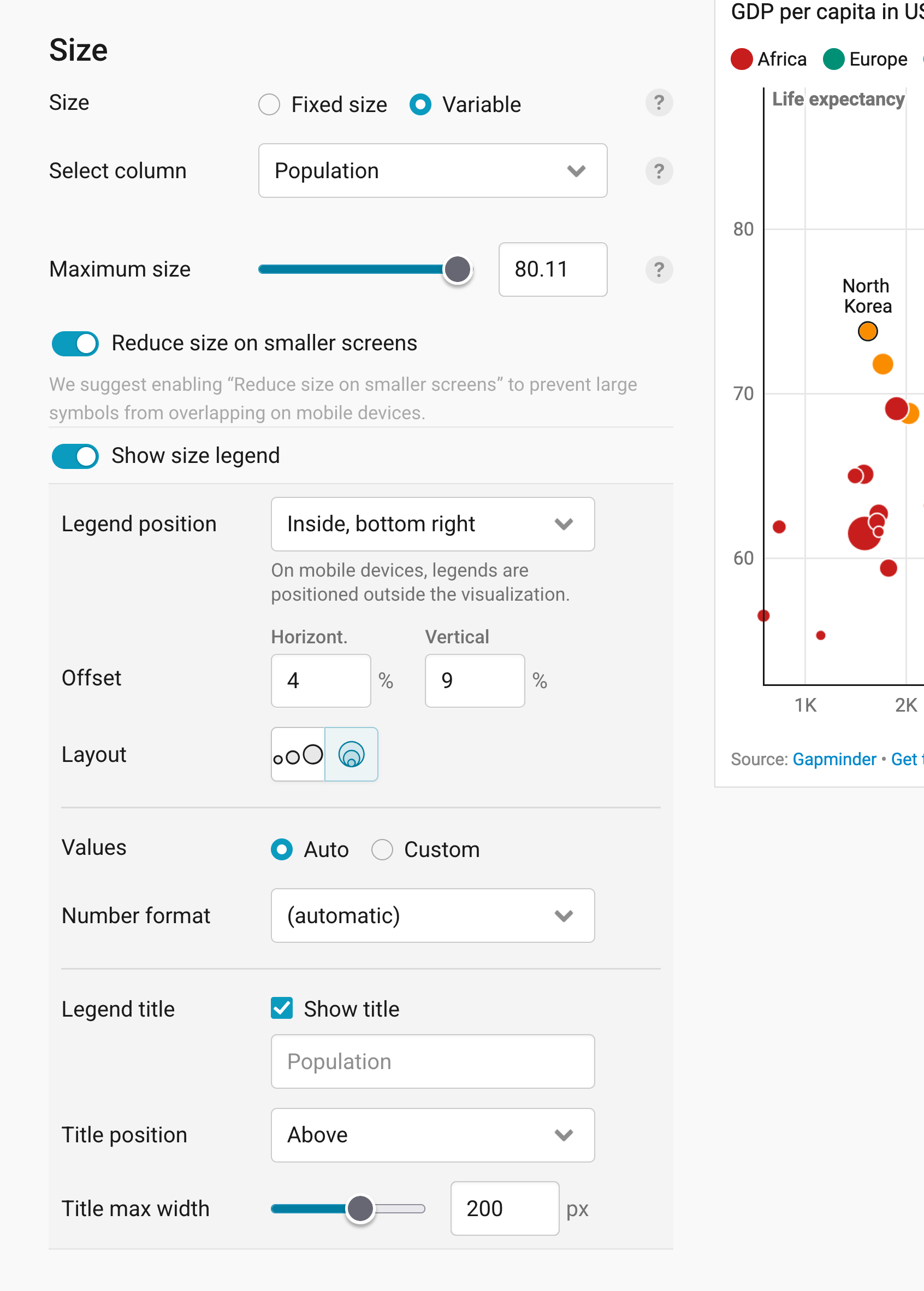
The Size panel lets you change the size of your dots:
- Size: gives all dots the same size (Fixed size, the default), which you can change with the slider below. With Variable, the size of each dot depends on a number column you choose under Select column, like "Population" in our chart. Maximum size then sets how big the biggest dot gets.
- Reduce size on smaller screens: makes your dots smaller on mobile, so they don't overlap as much. Datawrapper suggests turning it on once your dots have variable sizes.
- Show size legend: explains what the size of your dots means. Datawrapper recommends adding one, so readers know how to read the sizes. Here's what our size legend looks like with the settings you see in the screenshot above:
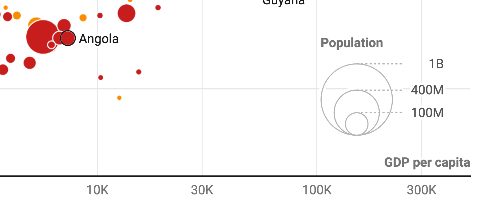
And here's what you can change in the settings:
- Legend position: places the size legend inside your chart, for example in the bottom right corner, or outside of it. On mobile, legends always appear outside the chart. With Offset, you can move it horizontally or vertically, as a share of the chart width and height.
- Layout: shows the circles of your size legend next to each other or nested inside each other.
- Values: lets Datawrapper pick which sizes the legend shows (Auto, the default), or lets you type in your own (Custom). Under Number format, you can decide how these values look.
- Legend title: shows a title for your size legend, like "Population" in our chart. You can change its text, its Title position, and how wide it can get before it breaks into the next line (Title max width).
Changing the shape
In the Shape panel, you can decide that your dots shouldn't be dots at all, but triangles or crosses, for example. With Fixed shape (the default), all dots get the shape you choose under Select shape (Circle by default). With Variable, their shape depends on a text column, like with the colors:
Adding a trend line
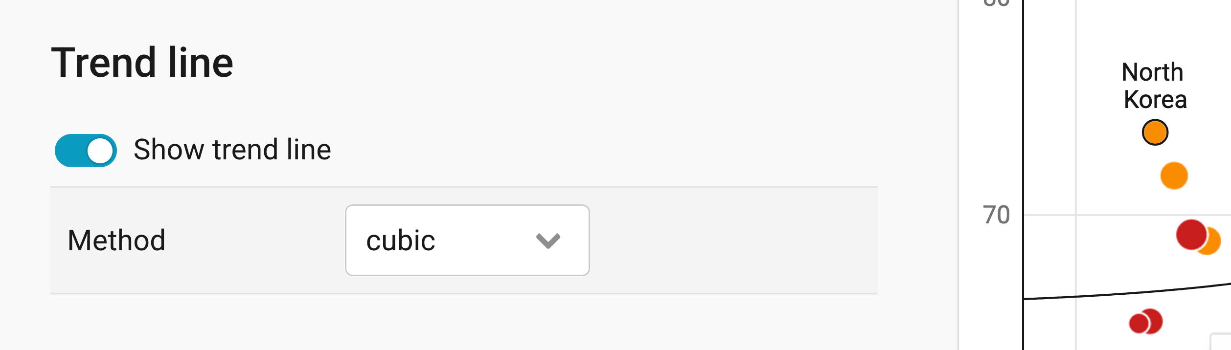
A trend line can help readers see the correlation between the two variables (in our case, GDP per capita and life expectancy). The line is calculated from the positions of the dots. It tells you two things: the direction and the strength of a correlation.
- A line rising from the lower left to the upper right (/) shows a positive correlation: when A increases, B increases, too.
- A line dropping from the upper left to the lower right (\) shows a negative correlation: when A increases, B decreases, and vice versa.
- The closer the dots sit to the line, the stronger the correlation.
- If the dots are scattered all over the place, don't use a trend line. There simply might be no correlation!
Turn on Show trend line to add a trend line to your scatter plot.
Under Method, choose how Datawrapper should calculate the line: linear, quadratic, cubic, power, logarithmic, or exponential. If your horizontal axis uses a log scale, a logarithmic trend line usually fits best. You can also draw your own line with custom line: Type in the Coordinates of the two points the line should connect, and tick unlimited to extend it across your whole chart.
Learn more about the different trend lines and how to choose one.
Here's what a scatter plot with a trend line looks like:
Changing the height

In the Appearance panel, you can set a fixed Plot height in pixels (300px by default), or one Based on width that scales with the width of your chart. Learn more about the difference between fixed and width-based plot heights.
That's it for the Refine tab. Let's move on to the Annotate tab:
Annotating your chart
Adding a title and source
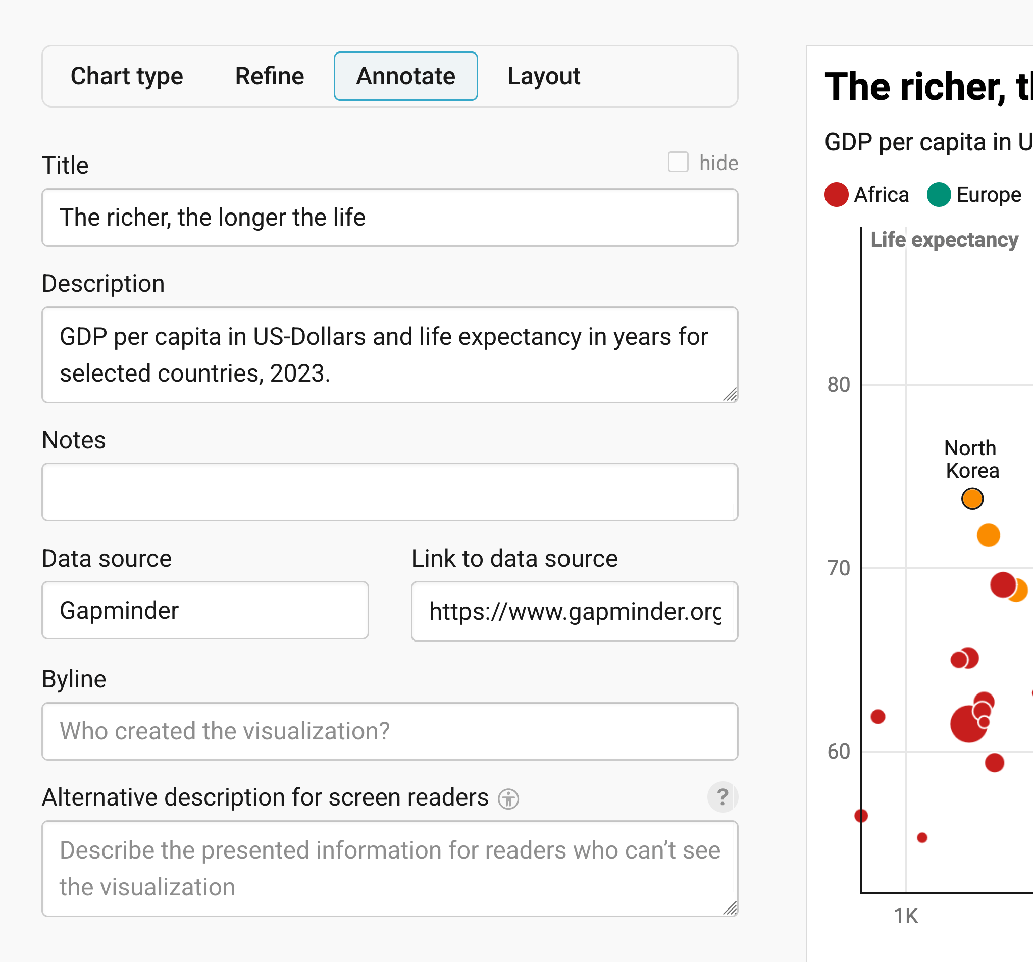
In the Annotate tab, you're first asked to give your visualization a title, description, notes, source, byline, and an alternative description for screen readers. You can find a detailed explanation of all these Annotate options here.
Adding text annotations

You can add annotations to your scatter plot by clicking on Add text annotation. You can then style and move the text, add an arrow and circle to it, and adjust how it will appear on mobile. In our chart, two text annotations point out the life expectancy in China and the USA. Here's an in-depth explanation of all the options.
Highlighting ranges
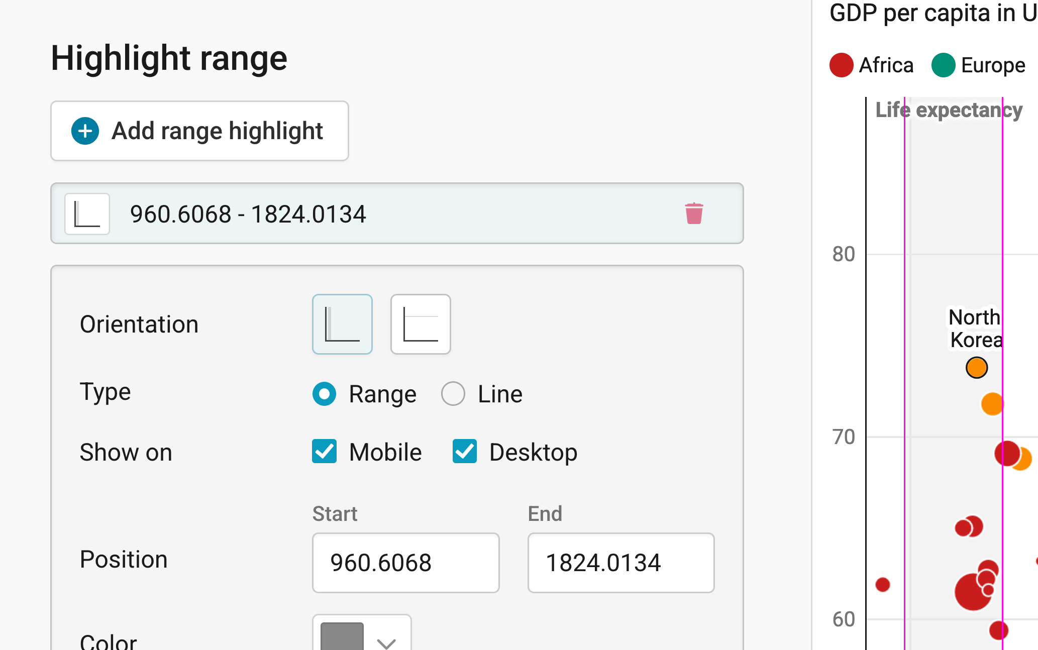
You can add range or line highlights to your chart by clicking on Add range highlight and then dragging on the chart where you want the highlight to be. You can then change its position, color, opacity, and line width and style, or delete it again. Here's an in-depth explanation of all the highlighting options.
Labeling dots
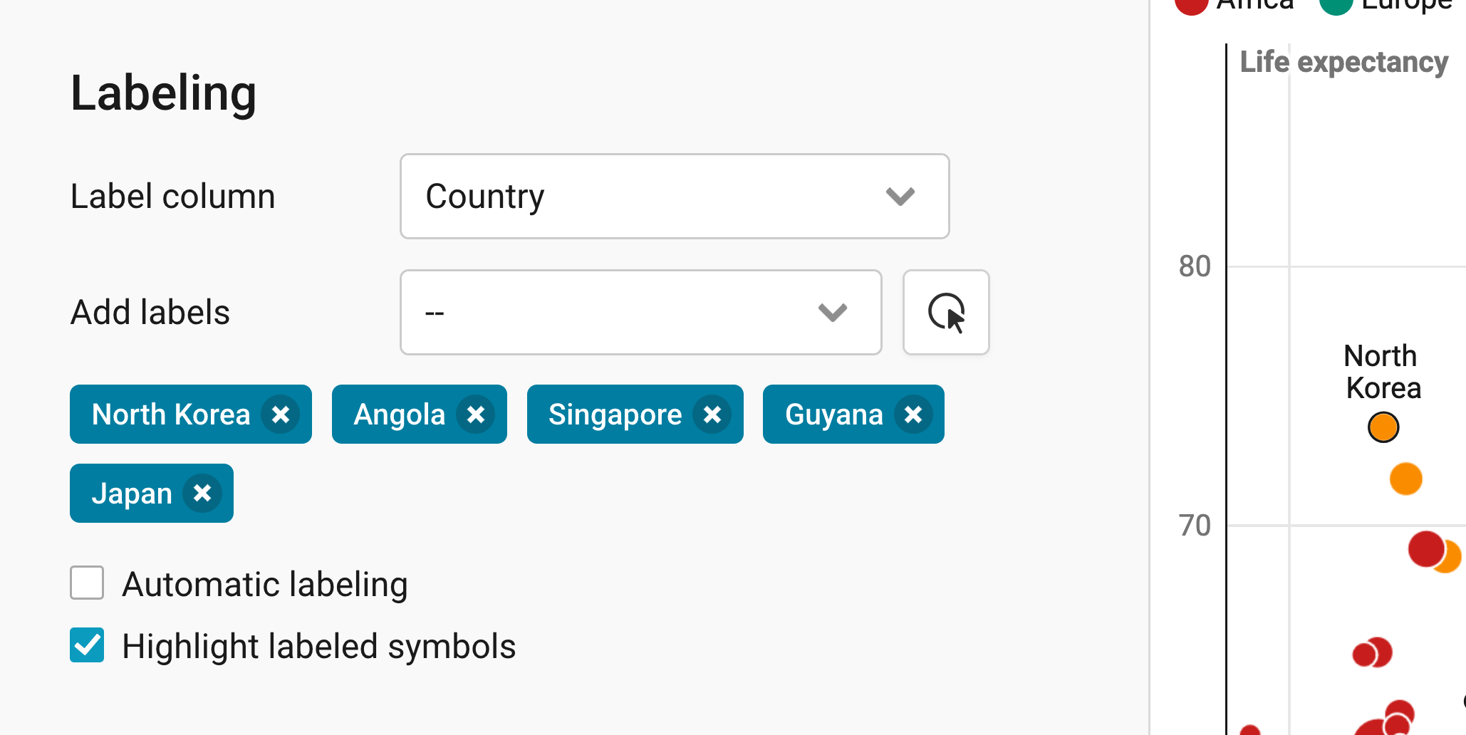
In the Labeling panel, you can decide whether your dots should be labeled. Under Label column, choose the column with the names of your dots. In most cases, that's the first column in your dataset, like "Country" in our data. You'll then get these options:
- Add labels: lets you choose dots that should always be labeled, either in the dropdown, or by clicking on the button next to it and then on the dots in your chart. To remove a label, click on the × next to its name. In our chart, we labeled North Korea, Angola, Singapore, Guyana, and Japan.
- Automatic labeling: lets Datawrapper label your dots automatically wherever there's space for a label, without overlapping other labels. On mobile, fewer labels will appear than on desktop.
- Highlight labeled symbols: makes it easier to see which label belongs to which dot.
Check your labels in the mobile view, too. Dots that sit far apart on desktop might end up right next to each other on a small screen, and their labels might overlap.
Customizing tooltips

Our scatter plots are interactive: When readers hover over a dot, more information can appear in a tooltip. In the Customize tooltip panel, you can decide which information will appear.
- Show tooltips: turns the tooltips on or off (on by default).
- Customize tooltips…: lets you write the title and text of your tooltips. You can use HTML and insert data columns, like
{{ country }}by clicking on one of the blue variables below the text box. In our chart, the tooltip shows the country as its title, followed by its GDP per capita and life expectancy. - Clicking makes tooltip stick: keeps the tooltip open when readers click on a dot, so they can e.g. click on a link in the tooltip.
Learn more about how to create tooltips.
Adding custom lines and areas
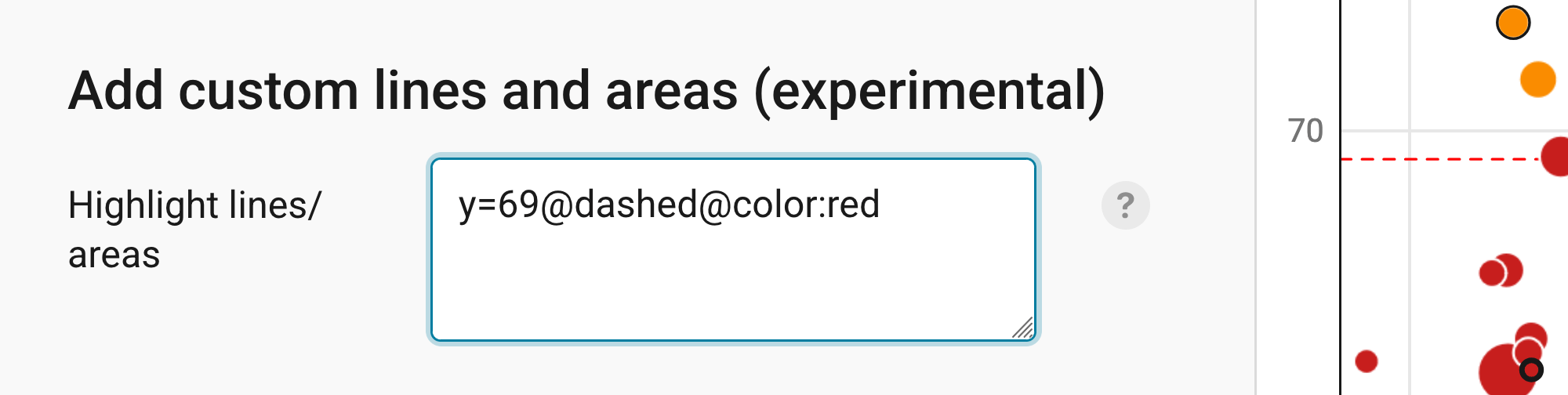
At the bottom of the Annotate tab, you can add extra lines and areas to your scatter plot. This feature is still experimental. It's helpful if you want to add a rectangle around or behind certain dots, or if you want to show a threshold line.
For example, writing "y=50" will create a horizontal line at the vertical axis point "50 years" (the same works for the horizontal axis, e.g. "x=2000").
You can create reference lines like these more easily with Add range highlight (see above). But to point out certain areas in your scatter plot, this feature can be really useful. Learn more about styling your custom lines and areas.
Publishing your chart
In the Layout tab, you can select an output locale, change the design theme and footer options, and enable social sharing. Find a detailed explanation of all the Layout options here.
In step 4: Publish & Embed, you can first publish your chart and then decide how it gets to your readers. We recommend pasting the embed code into your website or CMS, but you can also share the chart's URL. Learn more about both options here. To use your chart somewhere else, download it as a PNG (on any plan) or as an SVG or PDF (on paid plans). See what each plan includes on our pricing page.
And that's it! You've successfully created and customized a scatter plot.