How to create a grouped column chart
- Free
- Pro
- Business
- Enterprise
A grouped column chart shows values for multiple categories side by side, so you can compare them directly. This is ideal if you want to give a quick overview of something as you would with a bar chart or column chart, but add more information with the help of additional columns.
This tutorial will show you how to prepare your data to create and customize a grouped column chart.

Preparing your data
Formatting your data
To create this chart, your data needs the following structure:
- One header row containing descriptive labels ("Year", "Revenue", etc.)
- One column with categories. These can (but don't need to) be years, like in our case. Categories can be regions, products, etc.
- At least two columns containing numeric values. The values in these columns will determine the height of the bars for each category. In each group, there will be as many bars as columns with numeric values. Notice that you can also have negative values. Datawrapper will automatically scale the chart accordingly.
Below is part of the data we used to create the chart at the top of the page. You can find the whole data set in our data samples in step 1: Upload Data.
| Year | Revenue in mm. € | Net Profit in mm. € |
| 2004 | 647 | 138 |
| 2005 | 663 | 162 |
| 2006 | 749 | 249 |
| 2007 | 882 | 49 |
| 2008 | 957 | 184 |
| 2009 | 1059 | 196 |
| 2010 | 1291 | 202 |
| 2011 | 1070 | 36 |
| 2012 | 1166 | 89 |
| 2013 | 1386 | 72 |
| 2014 | 2096 | 141 |
Source: FIFA
Uploading your data
Once you have prepared your data, create a new chart in Datawrapper. You can do so by going to our homepage and clicking on Start creating. In step 1: Upload, you can copy & paste your dataset, upload it as a .csv or Excel file, or connect a Google Sheet. It will look like this:

Click Proceed at the bottom right to go to the next step.
Checking data and units
In the second step, you can check if your dataset was imported correctly and make changes to it, if necessary. If you did not upload a header row, you have to untick "First row as label" to avoid losing your first row of data. Always remember to do this if you don't have descriptive row and column headers.
In step 2, your data should look like the video below, automatically arranged in rows and columns. You can see that Datawrapper correctly recognized your numbers as numbers (and not as text or dates) because they are colored in blue and are right-aligned. To learn more about Datawrapper's automatic recognition of data formats, visit this article.
To create this chart in Datawrapper, you need to transpose the data, meaning you switch rows and columns:
To do so, you can click on the top left arrow button in the table, or on Swap rows and columns (transpose) below the table. To learn more about transposing, visit our article "Transposing a dataset".
To add a unit (like km/h, kg, inch, $, etc.) to your numbers, click on a column header and then add the unit of your choice to the Prepend/append options on the left. You can learn more about adding units to numbers here.
Click on Proceed at the bottom left to go to step 3: Visualize.
Choosing a grouped column chart
Under the tab Chart type, you will see a grid of chart types displayed. Your data will probably be displayed as a line chart at first. To change that, click on the Grouped Columns symbol in the grid:
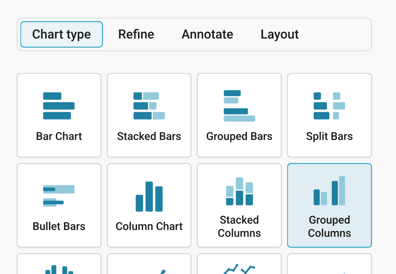
You will now see a grouped column chart, without a title, descriptions or customized colors. Next, you can refine, annotate, and customize this chart. Besides Chart type, you'll notice three more tabs in this step: Refine, Annotate, and Layout.
Refining your chart
Resizing
In any tab of step 3: Visualize, you can click, hold, and drag the arrow in the lower right corner to scale the chart window or manually determine the dimension of the chart by entering values in the boxes below the chart (Size).
We recommend checking what the chart looks like on different screen sizes multiple times while designing it, by clicking on the little icons (mobile, tablet, and computer) below the chart.
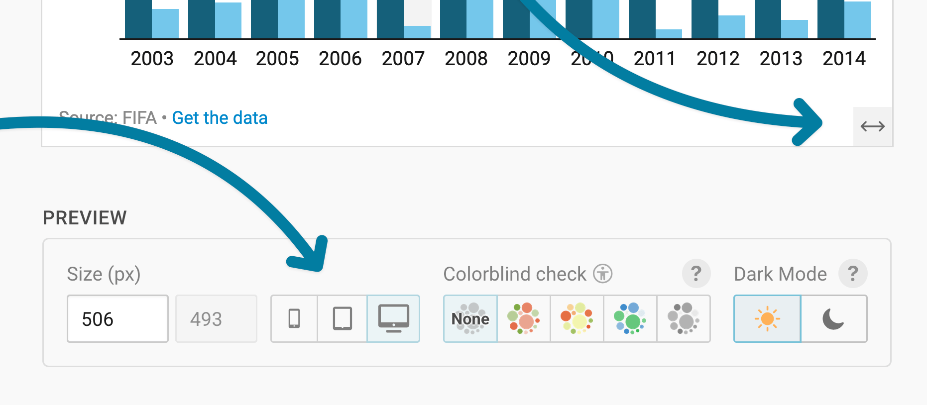
Learn more about changing the width and height of your chart in this article.
Changing the vertical axis
Let's continue with the Refine tab. Here, you see three panels: Vertical axis, Horizontal axis, and Appearance.
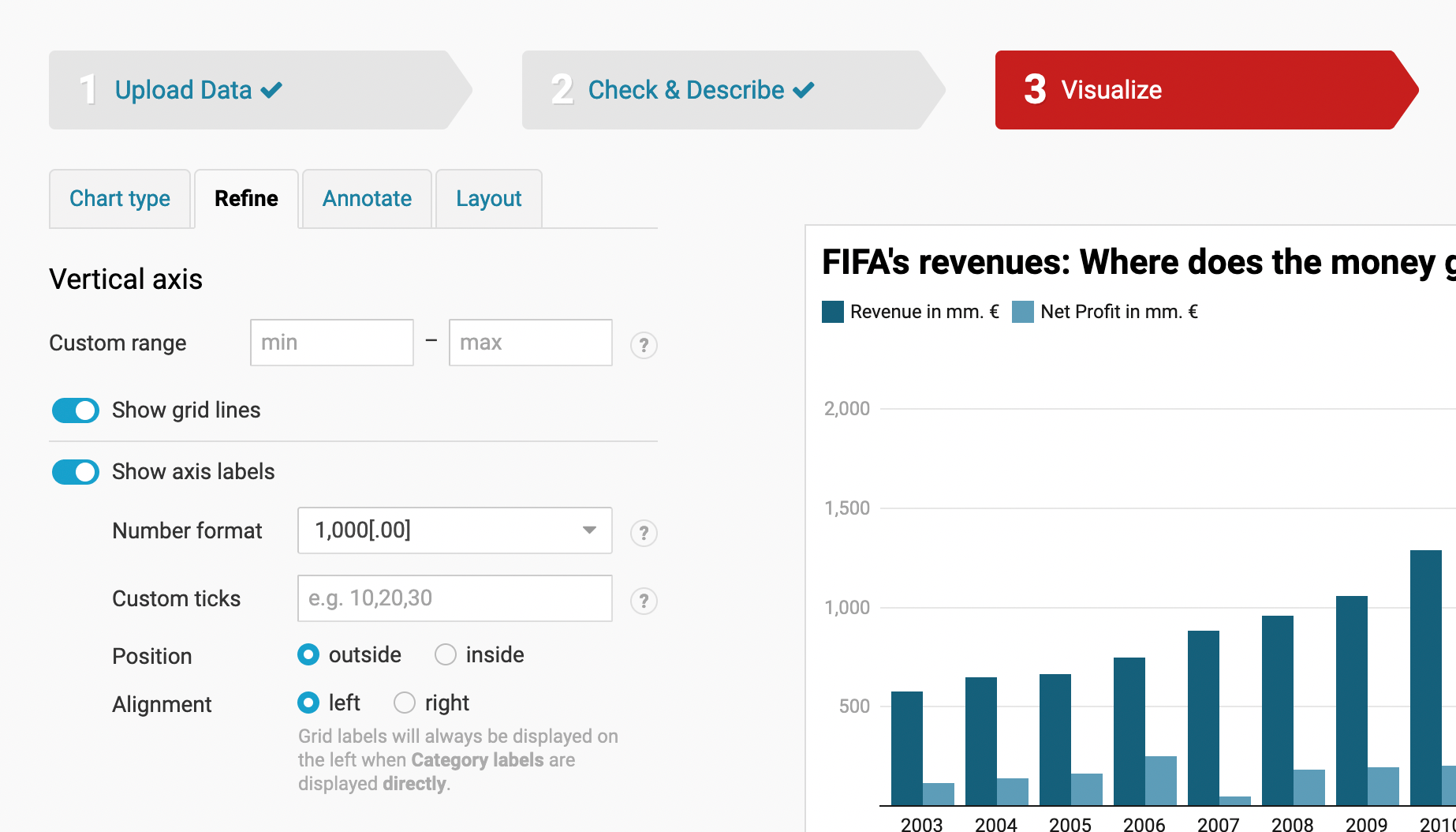
For the vertical axis, you can modify:
- custom range: allows you to set your own minimum and maximum values. However, please note that the vertical axis of a column chart has been set, by default, to start at zero, meaning that you can only modify the maximum value on this axis.
- show grid lines: depending on whether or not you want to highlight the display of certain values, you can choose to enable or disable this feature
- show axis labels: with the first setting Number format, you can decide how to show your values. Below are three examples but there are many different formats available and choice of a format ultimately depends on how big or small your values are:
- Choose the number format "123.4k" if you have big numbers like "1,303,428" that you'd rather display as "1.3m"
- Choose the number format "0.0" if you have very detailed numbers like "0.1922302" that you'd rather want to display as "0.2"
- Choose the number format "0%" or "0.0%" if you have a number that is a relative number. This setting will add a percentage sign.
Changing the horizontal axis
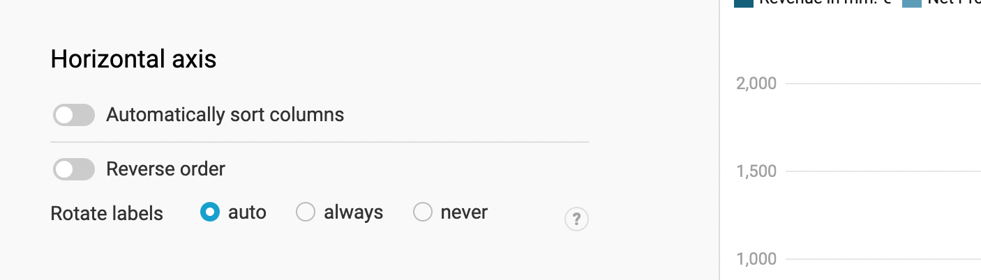
For the horizontal axis, you can:
- sort columns: here you have two settings; sort columns automatically and reverse the order. If you enable the automatic setting, your columns will be arranged in descending order and reversing the order would naturally sort them in ascending order.
- rotate labels: this handy little setting allows you to rotate the labels of your individual columns, in case some of the labels are too long to fit together horizontally. Here again, you have the choice to set the rotate option to ''auto'', ''always'' or ''never''.
Changing colors and appearance
The next option is Appearance. Here you have the option to adjust the colors of your bars. You can click on customize colors to assign each bar its own color. When you click on customize colors, you will have a list of labels displayed, together with a color box, depending on how many values you had. Click on a label (e.g. "net profit in mm.") and then on the color box below Choose a Color. A small popup will open, and you'll be able to choose a new color for your selected label.
You can also Reset all colors (to the right) or select all or none of the colors below the list of labels.
Below the customize color feature, you have more options: You can
- Show the color key above your chart, to let your readers know which bars belong to which category.
- Show or hide value labels. By default, we only show the value labels on the bars if readers hover over them. Here, you can decide to disable that or to always show the value labels.
Annotating your chart
Adding a title and source
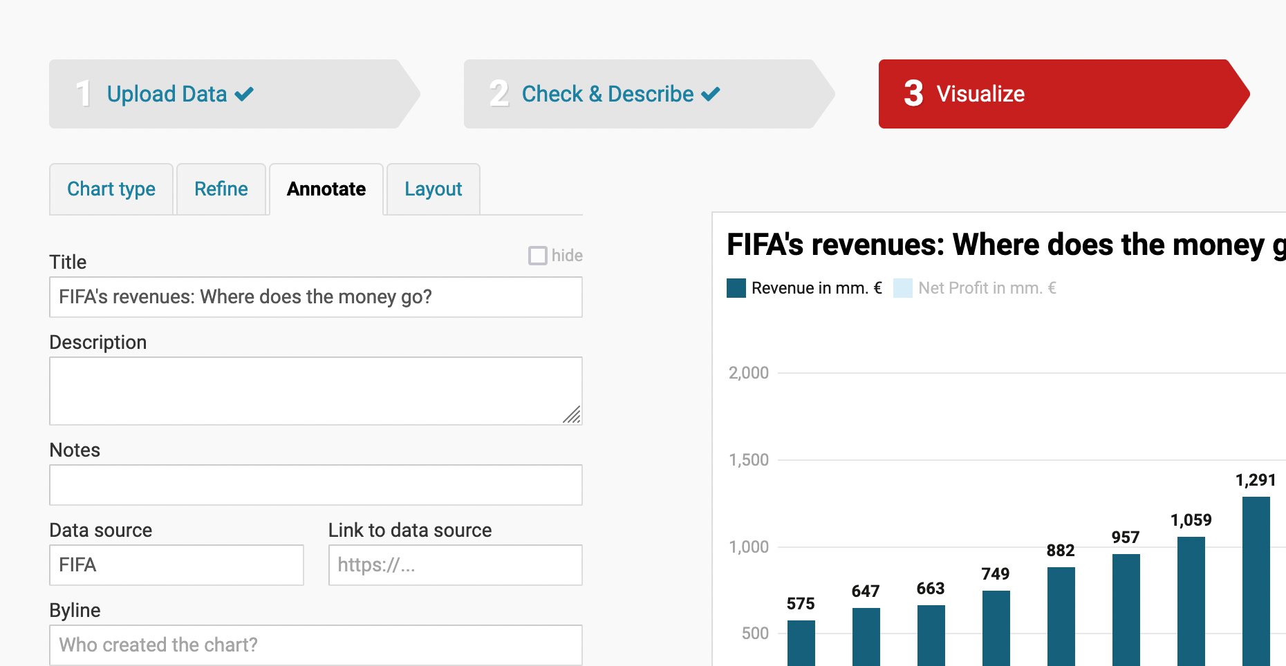
In the Annotate tab, you're first asked to give your visualization a title, description, notes, source, byline, and an alternative description for screen readers. You can find a detailed explanation of all these Annotate options here.
Highlighting columns
In the 2nd panel in the Annotate tab, you can emphasize certain categories. To do so, select the one(s) you want to highlight. The rest of the columns will automatically fade:
Adding text annotations
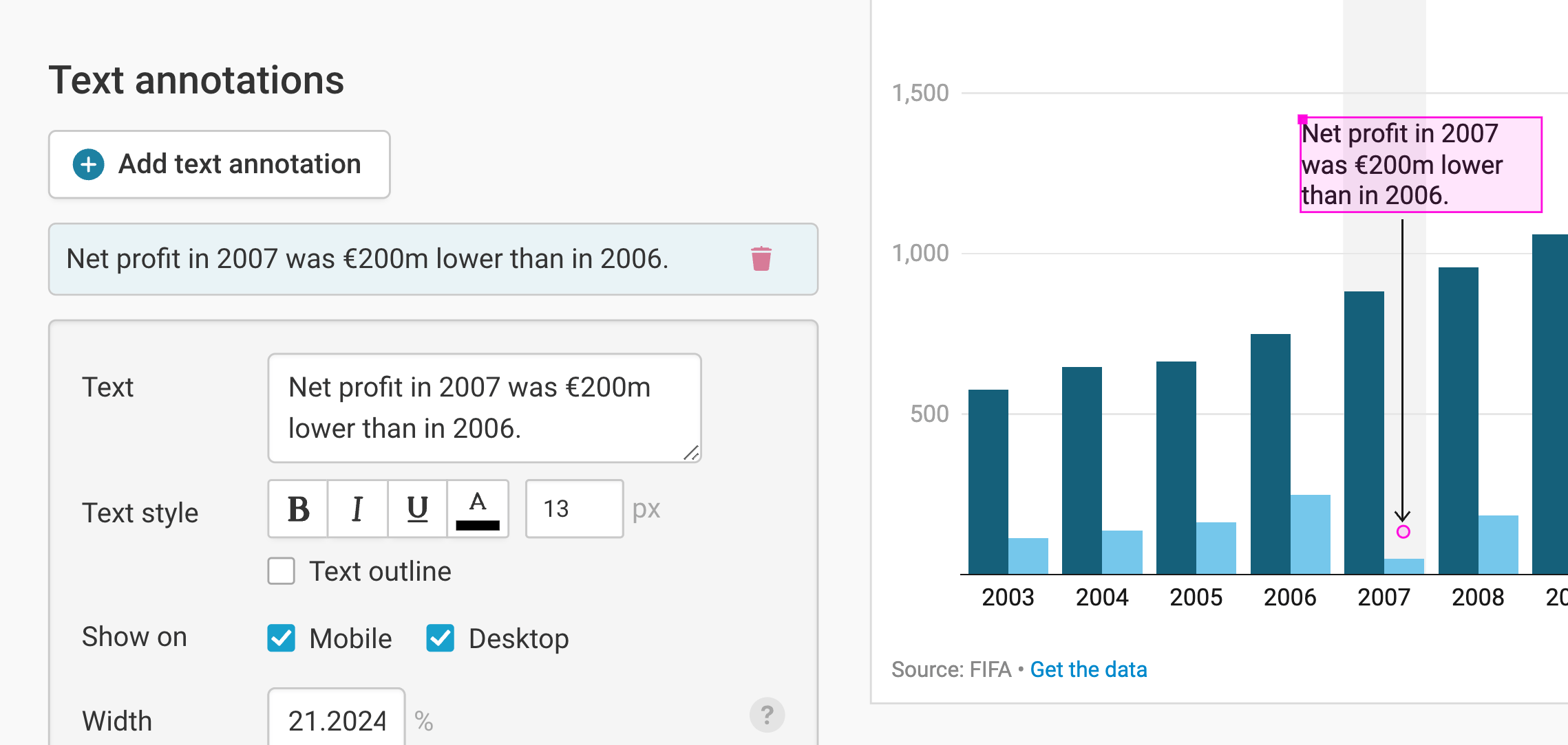
You can add annotations to your grouped column chart by clicking on Add text annotation. You can then style and move the text, add an arrow and circle to it, and adjust how it will appear on mobile. Here's an in-depth explanation of all the options.
Highlighting ranges
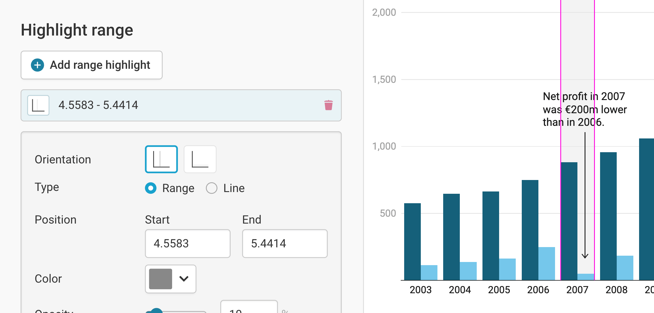
You can add range or line highlights to your chart by clicking on Add range highlight and then dragging on the chart where you want the highlight to be. You can then change its position, color, opacity, and line width and style, or delete it again. Here's an in-depth explanation of all the options.
Publishing your chart
In the Layout tab, you can select an output locale, change the design theme and footer options, and enable social sharing. Find a detailed explanation of all the Layout options here.
In step 4: Publish & Embed, you can first publish your chart and then decide how it gets to your readers. We recommend pasting the embed code into your website or CMS, but you can also share the chart’s URL. Learn more about both options here. To use your chart somewhere else, download it as a PNG (on any plan) or as an SVG or PDF (on paid plans). See what each plan includes on our pricing page.
And that's it! You've successfully created and customized your first grouped column chart.